
How to handle imbalanced text data in Natural Language Processing
Hello everyone today we are going to discuss an interesting problem with imbalanced text data.
We are interested to classify messages that are spam.
We are going to test different classification models such as Multinomial Naive Bayes, Random Forest (RF), XGBoost, Support Vector Machines (SVM), and different sampling and under-sampling methods such as Random over-sampling, SMOTE, and derivations, Random under-sampling techniques.
This example is helpful to show how to deal with this type of problem for your custom NLP problems.
What is Imbalanced Data?
Imbalanced data typically refers to a problem with classification problems where the classes are not represented equally.
There different performance measures that can give more insight into the accuracy of the model than traditional classification accuracy:
- Confusion Matrix: A breakdown of predictions into a table showing correct predictions (the diagonal) and the types of incorrect predictions made (what classes incorrect predictions were assigned).
- Precision: A measure of a classifiers exactness.
- Recall: A measure of a classifiers completeness
-
F1 Score (or F-score): A weighted average of precision and recall.
- Kappa (or Cohen’s kappa): Classification accuracy normalized by the imbalance of the classes in the data.
- ROC Curves: Like precision and recall, accuracy is divided into sensitivity and specificity and models can be chosen based on the balance thresholds of these values.
Step 1. Creation of the environment
I will create an environment called nlp, because I am interested in the Natural Language Processing (NLP) .
NLP enables computers to understand natural language as humans do. Whether the language is spoken or written, natural language processing uses artificial intelligence to take real-world input, process it, and make sense of it in a way a computer can understand.
First you need to install anaconda at this link
then after is installed type in your terminal
conda create -n nlp python==3.8
then
conda activate nlp
then in your terminal type the following commands:
conda install ipykernel
then we install
python -m ipykernel install --user --name nlp --display-name "Python (NLP)"
then we install the following libraries
pip install matplotlib seaborn nltk sklearn plotly wordcloud xgboost imbalanced-learn notebook jupyter
then we type
jupyter notebook
and we choose our Python (NLP) notebook.
We are interested to work in the problem of Spam Detection by using NLP.
In this project we are going to use a dataset contains messages that are spam and not.
You can download the dataset here.
Step 2. Load libraries
#importing necessary libraries
# General

import numpy as np
import pandas as pd
import re
import os
import pickle

# EDA

import matplotlib.pyplot as plt
import seaborn as sns
import plotly.express as px
from wordcloud import WordCloud
from collections import Counter

# NLP

import nltk
from nltk.corpus import stopwords
from nltk.stem.porter import PorterStemmer
from sklearn.feature_extraction.text import TfidfVectorizer
from nltk.tokenize import word_tokenize

# ML
from sklearn.pipeline import Pipeline
from sklearn.model_selection import train_test_split
from sklearn.naive_bayes import MultinomialNB
from sklearn.ensemble import RandomForestClassifier
from xgboost import XGBClassifier
from sklearn.svm import SVC
from sklearn.metrics import classification_report, confusion_matrix
Step 3. Data analysis
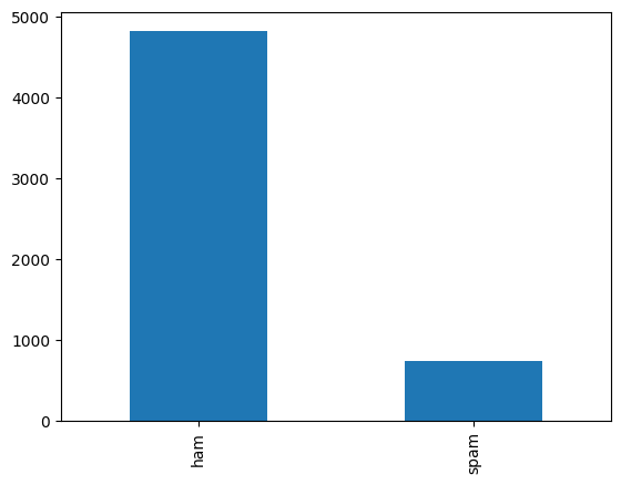
Here we need to analyze our dataset, first we read the dataset and then count how many messages are spam.
df=pd.read_csv('spam.csv',encoding = 'latin-1')
df.head()
| v1 | v2 | Unnamed: 2 | Unnamed: 3 | Unnamed: 4 | |
|---|---|---|---|---|---|
| 0 | ham | Go until jurong point, crazy.. Available only ... | NaN | NaN | NaN |
| 1 | ham | Ok lar... Joking wif u oni... | NaN | NaN | NaN |
| 2 | spam | Free entry in 2 a wkly comp to win FA Cup fina... | NaN | NaN | NaN |
| 3 | ham | U dun say so early hor... U c already then say... | NaN | NaN | NaN |
| 4 | ham | Nah I don't think he goes to usf, he lives aro... | NaN | NaN | NaN |
df['v1'].value_counts(dropna=False).plot(kind='bar')
Moreover we can get more information of our dataset by typing
df.info()
<class 'pandas.core.frame.DataFrame'>
RangeIndex: 5572 entries, 0 to 5571
Data columns (total 5 columns):
 #   Column      Non-Null Count  Dtype
---  ------      --------------  -----
 0   v1          5572 non-null   object
 1   v2          5572 non-null   object
 2   Unnamed: 2  50 non-null     object
 3   Unnamed: 3  12 non-null     object
 4   Unnamed: 4  6 non-null      object
dtypes: object(5)
memory usage: 217.8+ KB
or simply
df.describe()
| v1 | v2 | Unnamed: 2 | Unnamed: 3 | Unnamed: 4 | |
|---|---|---|---|---|---|
| count | 5572 | 5572 | 50 | 12 | 6 |
| unique | 2 | 5169 | 43 | 10 | 5 |
| top | ham | Sorry, I'll call later | bt not his girlfrnd... G o o d n i g h t . . .@" | MK17 92H. 450Ppw 16" | GNT:-)" |
| freq | 4825 | 30 | 3 | 2 | 2 |
#checking for null values
df.isnull().sum()
v1               0
v2               0
Unnamed: 2    5522
Unnamed: 3    5560
Unnamed: 4    5566
dtype: int64
#dropping the column with more null values
df.drop(['Unnamed: 2','Unnamed: 3','Unnamed: 4'],axis=1,inplace=True)
df.isnull().sum()
v1    0
v2    0
dtype: int64
#renaming the columns
df=df.rename({'v1':'label','v2':'text'},axis=1)
df.head()
| label | text | |
|---|---|---|
| 0 | ham | Go until jurong point, crazy.. Available only ... |
| 1 | ham | Ok lar... Joking wif u oni... |
| 2 | spam | Free entry in 2 a wkly comp to win FA Cup fina... |
| 3 | ham | U dun say so early hor... U c already then say... |
| 4 | ham | Nah I don't think he goes to usf, he lives aro... |
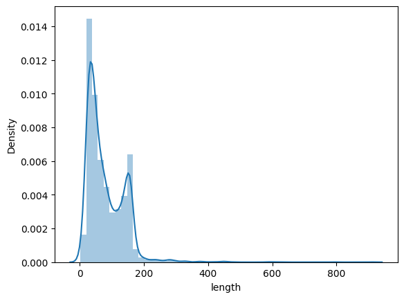
Calculating the length of each data sample. We will create a new length column that will show the length of each data sample. This new column will help us with preprocessing the data samples.
df['length'] = df['text'].apply(lambda x: len(x))
df.head()
| label | text | length | |
|---|---|---|---|
| 0 | ham | Go until jurong point, crazy.. Available only ... | 111 |
| 1 | ham | Ok lar... Joking wif u oni... | 29 |
| 2 | spam | Free entry in 2 a wkly comp to win FA Cup fina... | 155 |
| 3 | ham | U dun say so early hor... U c already then say... | 49 |
| 4 | ham | Nah I don't think he goes to usf, he lives aro... | 61 |
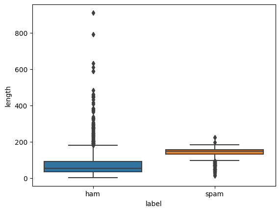
Distribution based on length of words
#analyzing text
df['length']=df['text'].apply(lambda x: len(x))
sns.distplot(df['length'], kde=True)
sns.boxplot(y='length', x='label', data=df)
df.head()
| label | text | length | |
|---|---|---|---|
| 0 | ham | Go until jurong point, crazy.. Available only ... | 111 |
| 1 | ham | Ok lar... Joking wif u oni... | 29 |
| 2 | spam | Free entry in 2 a wkly comp to win FA Cup fina... | 155 |
| 3 | ham | U dun say so early hor... U c already then say... | 49 |
| 4 | ham | Nah I don't think he goes to usf, he lives aro... | 61 |
Step 4. Data Preprocessing
NLTK has smaller sub-libraries that perform specific text cleaning tasks. These smaller libraries also have methods for text cleaning.
from nltk.stem import WordNetLemmatizer
from nltk import word_tokenize
import re
nltk.download('punkt')
Downloading stop words. We download the English stop words so that the model can identify the stop words in the texts and remove them.
nltk.download('stopwords')
nltk.download('omw-1.4')
We will use it to remove all the stop words in the dataset. We will then create custom functions for text cleaning and pass in the imported methods as parameters. To implement the custom functions, we will require Python regular expression (RegEx) module.
def convert_to_lower(text):
    return text.lower()
def remove_numbers(text):
    number_pattern = r'\d+'
    without_number = re.sub(pattern=number_pattern, repl=" ", string=text)
    return without_number

import string
def remove_punctuation(text):
    return text.translate(str.maketrans('', '', string.punctuation))

def remove_stopwords(text):
    removed = []
    stop_words = list(stopwords.words("english"))
    tokens = word_tokenize(text)
    for i in range(len(tokens)):
        if tokens[i] not in stop_words:
            removed.append(tokens[i])
    return " ".join(removed)
def remove_extra_white_spaces(text):
    single_char_pattern = r'\s+[a-zA-Z]\s+'
    without_sc = re.sub(pattern=single_char_pattern, repl=" ", string=text)
    return without_sc
def lemmatizing(text):
    lemmatizer = WordNetLemmatizer()
    tokens = word_tokenize(text)
    for i in range(len(tokens)):
        lemma_word = lemmatizer.lemmatize(tokens[i])
        tokens[i] = lemma_word
    return " ".join(tokens)
df['text_clean'] = df['text'].apply(lambda x: convert_to_lower(x))
df['text_clean'] = df['text_clean'].apply(lambda x: remove_numbers(x))
df['text_clean'] = df['text_clean'].apply(lambda x: remove_punctuation(x))
df['text_clean'] = df['text_clean'].apply(lambda x: remove_stopwords(x))
df['text_clean'] = df['text_clean'].apply(lambda x: remove_extra_white_spaces(x))
df['text_clean'] = df['text_clean'].apply(lambda x: lemmatizing(x))
df['length_after_cleaning'] = df['text_clean'].apply(lambda x: len(x))
df.head()
| label | text | length | text_clean | length_after_cleaning | |
|---|---|---|---|---|---|
| 0 | ham | Go until jurong point, crazy.. Available only ... | 111 | go jurong point crazy available bugis great wo... | 78 |
| 1 | ham | Ok lar... Joking wif u oni... | 29 | ok lar joking wif oni | 21 |
| 2 | spam | Free entry in 2 a wkly comp to win FA Cup fina... | 155 | free entry wkly comp win fa cup final tkts st ... | 101 |
| 3 | ham | U dun say so early hor... U c already then say... | 49 | u dun say early hor c already say | 33 |
| 4 | ham | Nah I don't think he goes to usf, he lives aro... | 61 | nah dont think go usf life around though | 40 |
#transform the values of the output variable into 0 and 1
#We can create the label map as follows:
label_map = {
    'ham': 0,
    'spam': 1,
}
df['label'] = df['label'].map(label_map)
Step 5. Implementing text vectorization
It converts the raw text into a format the NLP model can understand and use. Vectorization will create a numerical representation of the text strings called a sparse matrix or word vectors. The model works with numbers and not raw text. We will use TfidfVectorizer to create the sparse matrix.
from sklearn.feature_extraction.text import TfidfVectorizer
import numpy as np
tf_wb= TfidfVectorizer()
X_tf = tf_wb.fit_transform(df['text_clean'])
#Converting the sparse matrix into an array
#We then apply the toarray function to convert the sparse matrix into an array.
X_tf = X_tf.toarray()
X_tf.shape
X_train_tf, X_test_tf, y_train_tf, y_test_tf = train_test_split(X_tf, df['label'].values, test_size=0.3)
from sklearn.naive_bayes import GaussianNB
NB = GaussianNB()
NB.fit(X_train_tf, y_train_tf)
NB_pred= NB.predict(X_test_tf)
print(NB_pred)
from sklearn.metrics import accuracy_score
print(accuracy_score(y_test_tf, NB_pred))
[0 0 0 ... 0 0 0]
0.8767942583732058
from imblearn.over_sampling import RandomOverSampler
We will use the RandomOverSampler function to balance the classes.
RandomOverSampler will increase the data samples in the minority class (spam). It makes the minority class have the same data samples as the majority class (ham). The function synthesizes new dummy data samples in the minority class to enable class balancing.
X_train, X_test, y_train, y_test = train_test_split(df['text_clean'], df['label'].values, test_size=0.30)
After splitting the dataset, we will use the Counter module to check the number of data samples in the majority and minority classes. We import the module as follows:
from collections import Counter
Counter(y_train)
Counter({0: 3391, 1: 509})
#Vectorizing the X_train
vectorizer = TfidfVectorizer()
vectorizer.fit(X_train)
The fit function will fit the initialized TfidfVectorizer function to the X_train. We then use the transform function to apply the vectorization method.
X_train_tf = vectorizer.transform(X_train)
We finally convert the transformed text (sparse matrix) to an array as follows:
X_train_tf = X_train_tf.toarray()
#Vectorizing the X_test
X_test_tf = vectorizer.transform(X_test)
X_test_tf = X_test_tf.toarray()
Let’s now apply the RandomOverSampler function.
Applying RandomOverSampler function We use the following code:
ROS = RandomOverSampler(sampling_strategy=1)
The function uses the sampling_strategy parameter to balance the class. We set the parameter’s value to 1 to ensure the dataset classes have 1:1 data samples. We then apply the function to the training set. It will generate the new data samples to ensure both classes are balance
X_train_ros, y_train_ros = ROS.fit_resample(X_train_tf, y_train)
Let’s recheck the number of data samples in the majority and minority classes:
Counter(y_train_ros)
Counter({0: 3391, 1: 3391})
Using the balanced dataset to build the same model
nb = GaussianNB()
nb.fit(X_train_ros, y_train_ros)
y_preds = nb.predict(X_test_tf)
print(y_preds)
[0 0 1 ... 0 0 0]
print(accuracy_score(y_test, y_preds))
0.8851674641148325
Actually NLP is one of the most common areas in which resampling of data is needed as there are many text classification tasks dealing with imbalanced problem (think of spam filtering, insulting comment detection, article classification, etc.
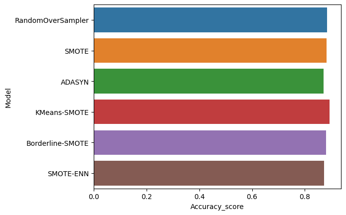
Step 6. Oversampling
Synthetic Minority Oversampling Technique (SMOTE) is a statistical technique for increasing the number of cases in your dataset in a balanced way. The component works by generating new instances from existing minority cases that you supply as input.
X_tf.shape
(5572, 7858)
from imblearn.over_sampling import SMOTE, KMeansSMOTE , ADASYN,SVMSMOTE,KMeansSMOTE,BorderlineSMOTE
from imblearn.combine import SMOTEENN, SMOTETomek
from imblearn.metrics import classification_report_imbalanced
def run_model(X,y,model):
    X_train, X_test, y_train, y_test = train_test_split(X, y, test_size=0.30)
    print(Counter(y_train))
    vectorizer_smote = TfidfVectorizer()
    vectorizer_smote.fit(X_train)
    #Vectorizing the X_train
    X_train_vec = vectorizer_smote.transform(X_train)
    X_train_vec = X_train_vec.toarray()
    #Vectorizing the X_test
    X_test_vec = vectorizer_smote.transform(X_test)
    X_test_vec = X_test_vec.toarray()
    # transform the dataset
    oversample = model
    X_train_over, y_train_over = oversample.fit_resample(X_train_vec, y_train)
    print(Counter(y_train_over))
    nb = GaussianNB()
    nb.fit(X_train_over, y_train_over)
    y_preds = nb.predict(X_test_vec)
    score = accuracy_score(y_test,y_preds)
    print("Accuracy: ",score)
    #target_names = ['class 0', 'class 1']
    #print(classification_report_imbalanced(y_test, y_preds,     target_names=target_names))
    return score
X=df['text_clean']
y=df['label'].values
#Object to over-sample the minority class(es) by picking samples at random with replacement.
oversample= RandomOverSampler(sampling_strategy=1)
ov1=run_model(X,y,model=oversample)
Counter({0: 3353, 1: 547})
Counter({0: 3353, 1: 3353})
Accuracy:  0.8839712918660287
# over-sampling using SMOTE.
oversample=SMOTE(sampling_strategy=0.2)
ov2=run_model(X,y,model=oversample)
Counter({0: 3389, 1: 511})
Counter({0: 3389, 1: 677})
Accuracy:  0.882177033492823
#Oversample using Adaptive Synthetic (ADASYN) algorithm.
oversample = ADASYN()
ov3=run_model(X,y,model=oversample)
Counter({0: 3375, 1: 525})
Counter({1: 3399, 0: 3375})
Accuracy:  0.8708133971291866
#KMeans clustering before to over-sample using SMOTE.
oversample=KMeansSMOTE()
ov4=run_model(X,y,model=oversample)
Counter({0: 3391, 1: 509})
Counter({1: 3391, 0: 3391})
Accuracy:  0.8929425837320574
#Over-sampling using Borderline SMOTE
oversample=BorderlineSMOTE()
ov5=run_model(X,y,model=oversample)
Counter({0: 3376, 1: 524})
Counter({0: 3376, 1: 3376})
Accuracy:  0.8803827751196173
#Over-sampling using SMOTE and cleaning using ENN.
oversample=SMOTEENN()
ov6=run_model(X,y,model=oversample)
Counter({0: 3376, 1: 524})
Counter({0: 3361, 1: 3352})
Accuracy:  0.8738038277511961
#Over-sampling using SVM-SMOTE.
oversample=SVMSMOTE()
ov7=run_model(X,y,model=oversample)
Counter({0: 3391, 1: 509})
Counter({0: 3391, 1: 3391})
Accuracy:  0.882177033492823
over_models = pd.DataFrame({
    'Model':['RandomOverSampler',
             'SMOTE',
             'ADASYN',
             'KMeans-SMOTE',
             'Borderline-SMOTE',
             'SMOTE-ENN'
            ],
    'Accuracy_score' :[ov1 ,ov2, ov3, ov4,ov5,ov6
                      ]
})
sns.barplot(x='Accuracy_score', y='Model', data=over_models)
over_models.sort_values(by='Accuracy_score', ascending=False)
| Model | Accuracy_score | |
|---|---|---|
| 3 | KMeans-SMOTE | 0.892943 |
| 0 | RandomOverSampler | 0.883971 |
| 1 | SMOTE | 0.882177 |
| 4 | Borderline-SMOTE | 0.880383 |
| 5 | SMOTE-ENN | 0.873804 |
| 2 | ADASYN | 0.870813 |
- Some researchers have investigated whether SMOTE is effective on high-dimensional or sparse data, such as data used in text classification or genomics datasets. This paper has a good summary of the effects and of the theoretical validity of applying SMOTE in such cases: Blagus and Lusa: SMOTE for high-dimensional class-imbalanced data.
- If SMOTE is not effective other approaches that you might consider include:
- Methods for oversampling the minority cases or undersampling the majority cases.
- Ensemble techniques that help the learner directly by using clustering, bagging, or adaptive boosting.
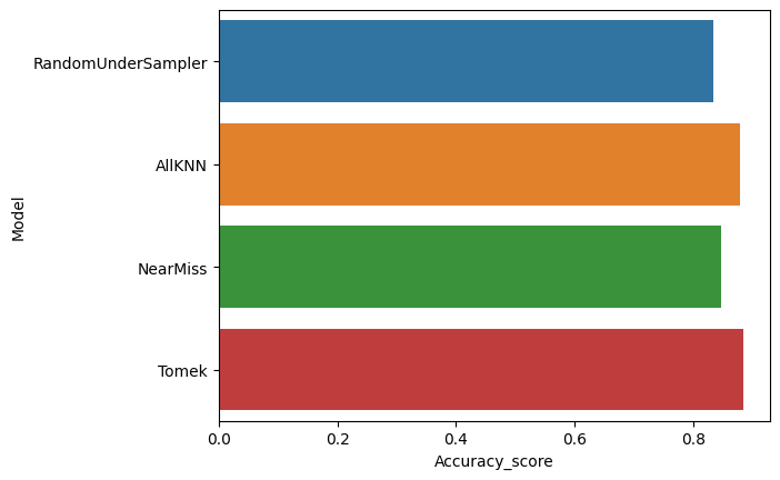
Step 7. Downsampling
from imblearn.under_sampling import RandomUnderSampler,AllKNN,NearMiss, TomekLinks
# random under-sampling
undersample=RandomUnderSampler()
un1=run_model(X,y,model=undersample)
Counter({0: 3393, 1: 507})
Counter({0: 507, 1: 507})
Accuracy:  0.8331339712918661
# Undersample based on the AllKNN method.
undersample=AllKNN()
un2=run_model(X,y,model=undersample)
Counter({0: 3373, 1: 527})
Counter({0: 3370, 1: 527})
Accuracy:  0.8779904306220095
# under-sampling based on NearMiss methods.
# NearMiss-1: Majority class examples with minimum average distance to three closest minority class examples.
undersample=NearMiss(version=1)
un3=run_model(X,y,model=undersample)
Counter({0: 3395, 1: 505})
Counter({0: 505, 1: 505})
Accuracy:  0.8462918660287081
#Under-sampling by removing Tomek's links.
undersample=TomekLinks()
un4=run_model(X,y,model=undersample)
Counter({0: 3385, 1: 515})
Counter({0: 3383, 1: 515})
Accuracy:  0.8845693779904307
under_models = pd.DataFrame({
    'Model':['RandomUnderSampler',
             'AllKNN',
             'NearMiss',
             'Tomek'
            ],
    'Accuracy_score' :[un1 ,un2, un3, un4,
                      ]
})
sns.barplot(x='Accuracy_score', y='Model', data=under_models)
under_models.sort_values(by='Accuracy_score', ascending=False)
| Model | Accuracy_score | |
|---|---|---|
| 3 | Tomek | 0.884569 |
| 1 | AllKNN | 0.877990 |
| 2 | NearMiss | 0.846292 |
| 0 | RandomUnderSampler | 0.833134 |
Step 8. Oversampling Pipeline
TF-IDF - normalizing and weighting with diminishing importance tokens that occur in the majority of documents.
1.TF(Term frequency)-Term frequency works by looking at the frequency of a particular term you are concerned with relative to the document. There are multiple measures, or ways, of defining frequency
2.IDF (inverse document frequency)-Inverse document frequency looks at how common (or uncommon) a word is amongst the corpus.
The output above shows the label column has the assigned integer values (0 and 1). The next step is to implement text vectorization.
We will split the vectorized dataset into two portions/sets. The first portion will be for model training and the second portion for model testing. We will use the train_test_split method to split the vectorized dataset.
#split the data into train and test sets
X=df['text_clean']
y=df['label']
#y=df['label']
X_train, X_test, y_train, y_test = train_test_split(X,y,test_size = 0.2, random_state = 42)
def model(model_name,X_train,y_train,X_test,y_test):
    pipeline=Pipeline([
    ('tfidf', TfidfVectorizer()),#transform the texts into the vectorized input variables X
    ('model', model_name),
    ])
    pipeline.fit(X_train,y_train)

    preds=pipeline.predict(X_test)

    print (classification_report(y_test,preds))
    print (confusion_matrix(y_test,preds))
    print('Accuracy:', pipeline.score(X_test, y_test)*100)
    print("Training Score:",pipeline.score(X_train,y_train)*100)
    from sklearn.metrics import accuracy_score
    score = accuracy_score(y_test,preds)
    return score
MultinomialNB
mnb=model(MultinomialNB(),X_train,y_train,X_test,y_test)
              precision    recall  f1-score   support

           0       0.96      1.00      0.98       965
           1       1.00      0.75      0.85       150

    accuracy                           0.97      1115
   macro avg       0.98      0.87      0.92      1115
weighted avg       0.97      0.97      0.96      1115

[[965   0]
 [ 38 112]]
Accuracy: 96.59192825112108
Training Score: 97.55440879515369
RF
rf=model(RandomForestClassifier(),X_train,y_train,X_test,y_test)
              precision    recall  f1-score   support

           0       0.97      1.00      0.99       965
           1       1.00      0.83      0.91       150

    accuracy                           0.98      1115
   macro avg       0.99      0.92      0.95      1115
weighted avg       0.98      0.98      0.98      1115

[[965   0]
 [ 25 125]]
Accuracy: 97.75784753363229
Training Score: 100.0
XGBoost
xgb=model(XGBClassifier(),X_train,y_train,X_test,y_test)
              precision    recall  f1-score   support

           0       0.97      1.00      0.98       965
           1       0.97      0.82      0.89       150

    accuracy                           0.97      1115
   macro avg       0.97      0.91      0.94      1115
weighted avg       0.97      0.97      0.97      1115

[[961   4]
 [ 27 123]]
Accuracy: 97.21973094170404
Training Score: 98.99035225487997
SVM
svc=model(SVC(),X_train,y_train,X_test,y_test)
              precision    recall  f1-score   support

           0       0.97      1.00      0.99       965
           1       0.98      0.83      0.90       150

    accuracy                           0.98      1115
   macro avg       0.98      0.92      0.94      1115
weighted avg       0.98      0.98      0.97      1115

[[963   2]
 [ 25 125]]
Accuracy: 97.57847533632287
Training Score: 99.73076060130133
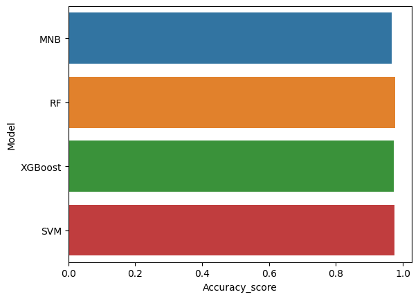
Model Comparison
models = pd.DataFrame({
    'Model':['MNB','RF','XGBoost', 'SVM'],
    'Accuracy_score' :[mnb ,rf, xgb, svc]
})
sns.barplot(x='Accuracy_score', y='Model', data=models)
models.sort_values(by='Accuracy_score', ascending=False)
| Model | Accuracy_score | |
|---|---|---|
| 1 | RF | 0.977578 |
| 3 | SVM | 0.975785 |
| 2 | XGBoost | 0.972197 |
| 0 | MNB | 0.965919 |
Step 9 Final model
def run_model_sampling(X,y,mlmodel,sampling=None):
    X_train, X_test, y_train, y_test = train_test_split(X, y, test_size=0.30)
    print(Counter(y_train))
    vectorizer_smote = TfidfVectorizer()
    vectorizer_smote.fit(X_train)
    #Vectorizing the X_train
    X_train_vec = vectorizer_smote.transform(X_train)
    X_train_vec = X_train_vec.toarray()
    #Vectorizing the X_test
    X_test_vec = vectorizer_smote.transform(X_test)
    X_test_vec = X_test_vec.toarray()
    # transform the dataset ( Sampling model)
    oversample = sampling
    if oversample:
        X_train_over, y_train_over = oversample.fit_resample(X_train_vec, y_train)
        X_train_vec= X_train_over
        y_train = y_train_over
    print(Counter(y_train))
    # Machine Learning Model
    model=mlmodel
    model.fit(X_train_vec, y_train)
    y_preds = model.predict(X_test_vec)
    score = accuracy_score(y_test,y_preds)
    print("Accuracy: ",score)
    target_names = ['class 0', 'class 1']
    print(classification_report_imbalanced(y_test, y_preds, target_names=target_names))
    return score
X=df['text_clean']
y=df['label'].values
mlmodel=RandomForestClassifier()
sampling=KMeansSMOTE()
run_model_sampling(X,y,mlmodel,sampling)
Counter({0: 3364, 1: 536})
Counter({0: 3364, 1: 3364})
Accuracy:  0.9736842105263158
                   pre       rec       spe        f1       geo       iba       sup

    class 0       0.97      1.00      0.79      0.99      0.89      0.81      1461
    class 1       1.00      0.79      1.00      0.88      0.89      0.77       211

avg / total       0.97      0.97      0.82      0.97      0.89      0.80      1672

0.9736842105263158
X=df['text_clean']
y=df['label'].values
mlmodel=RandomForestClassifier()
run_model_sampling(X,y,mlmodel)
Counter({0: 3390, 1: 510})
Counter({0: 3390, 1: 510})
Accuracy:  0.9766746411483254
                   pre       rec       spe        f1       geo       iba       sup

    class 0       0.97      1.00      0.84      0.99      0.91      0.85      1435
    class 1       1.00      0.84      1.00      0.91      0.91      0.82       237

avg / total       0.98      0.98      0.86      0.98      0.91      0.85      1672


0.9766746411483254
As we see the oversampling/ downsampling in general, does not provide better accuracy for this current set of data. What we have learned is that is better to choose a better machine learning model than apply sampling methods. And also the cleaning of the data provides a big improvement in the NLP accuracy
Actually NLP is one of the most common areas in which resampling of data is needed as there are many text classification tasks dealing with imbalanced problem but SMOTE seem to be problematic here for some reasons: SMOTE works in feature space. It means that the output of SMOTE is not a synthetic data which is a real representative of a text inside its feature space. On one side SMOTE works with KNN and on the other hand, feature spaces for NLP problem are dramatically huge. KNN will easily fail in those huge dimensions.
Do not care about the real text representation of new synthetic samples. You need to balance the distribution for your classifier not for a reader of text data. In principle we can use SMOTE as traditional with some Dimensionality Reduction step. 1) Lets assume you want to make your data samples from minor class double using K-NN. Ignore the major class(es) and keep only minor class samples. 2) Ignore the major class. Get a length distribution of all documents in minor class so that we generate new samples according the the true document length (number of words/phrases).
Well I hope was helpful the discussion, you can download this notebook here
Congratulations! You have practiced how to classify messages by using different NLP methods.
Leave a comment