Speech Recognition with Convolution Neural Networks
Hello everyone, today we are going to discuss how to build a Neural Network to detect speech words using Tensorflow.
![]()
We are going to build a neural network using Convolutional Neural Networks.
In the previous blog post we have studied this case by using Pytorch with LSTM Recurrent Neural Network here.
In this post we are going to download several sounds that will be used to create your Machine Learning Model.
The goal of this project is to implement an audio classification system, which:
- Reads in an audio clip (containing at most one word),
- Recognizes the class(label) of this audio.
Classes
10 classes are chosen, namely:
classes=["yes", "no", "up", "down", "left", "right", "on", "off", "stop", "go"]
Introduction
In ordering to understand the sound, it is important to know that the wave equation for sound in three dimensions may be depicted as
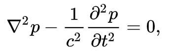
where squared nabla is the Laplace operator and p is the acoustic pressure the local deviation from the ambient pressure, and c is the speed of sound. The solution of this equation give us the wave function of the sound. For example is three dimensions, from a point source is best described in spherical polar equation
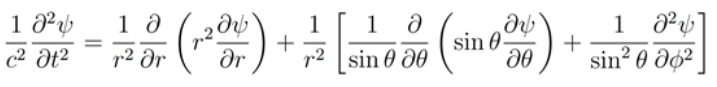
with the wave form
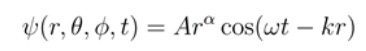
Waves in three-dimensions from a point source is best described in spherical polar coordinates.
One dimensions you can have the wave form like the following.
You can download python code here.
RNN vs CNN
Convolutional Neural Networks it is well known for the community of computer vision to deal problems regarding to images. However depending of the nature of the problem sometimes the CNN may be also used in other fields of research such as audio classification like I will shown in this blog post.
Let us discuss some differences between RNN and CNN.
Comparison:
- CNN reuses parameters in the space dimension – same kernel, every location
- RNN reuses parameters in the time dimension – same parameters, every time step
Long short-term memory (LSTM)
Problems with vanilla RNN:
- It’s difficult to retain memory for a long time
- It has the vanishing gradient problem
Long short-term memory (LSTM) was proposed to address these problem
An LSTM unit is composed of:
- A cell
- An input gate
- An output gate
- A forget gate
Long short-term memory (LSTM)
The core idea:
- Cell states: carry over memory information
- Input gate: let input affect the memory
- Output gate: let memory affect output
- Forget gate: throw away the memory
- With the forget gate, we can learn to forget
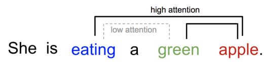
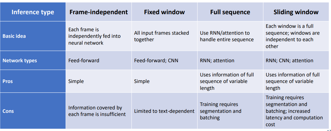
Given an input sequence
• RNN produces an output for each input
• The output sequence has the same length as the input sequence
For speaker recognition:
• We need a single embedding
Convolution Neural Network
The innovation of using the convolution operation in a neural network is that the values of the filter are weights to be learned during the training of the network.
The network will learn what types of features to extract from the input. Specifically, training under stochastic gradient descent, the network is forced to learn to extract features from the matrix that minimize the loss for the specific task the network is being trained to solve, e.g. extract features that are the most useful for classifying.
In pure mathematical terms, a convolution represents the blending of two functions, f(x) and g(x), as one slides over the other.
Fig. Convolution of two functions, f and g.
Convolution is performed by sliding a small array of numbers, typically a matrix of size [nxm] sequentially over different portions of the picture.
This convolution matrix is also known as a convolution filter or kernel. For each position of the convolution matrix, the corresponding scalar values are multiplied and added together to replace the original scalar value of the matrix. In this way the values of the neighboring values of the array are blended together with that of the central value of the array to created a convolved feature matrix.
In other words, is a simple matrix multiplication where the kernel matrix modify the values of the original matrix to emphasize details of certain properties of the original matrix.
Let us summarize some of the different aspects of the RNN vs CONV
Setup the environment
The Python environment that we will use is Keras that is explained in this blog post here.
In addition we require the following libraries
pip install librosa tqdm shutil pathlib
Step 1 Import the packages
from time import sleep
from tqdm import tqdm
import os
import urllib.request
import pathlib
import shutil
import os
import librosa
import IPython.display as ipd
import matplotlib.pyplot as plt
import numpy as np
from scipy.io import wavfile
import warnings
warnings.filterwarnings("ignore")
Step 2 Creation of some utility programs
We define some functions that allow us download the datasets that we need to use to create our ML model and train it.
class DownloadProgressBar(tqdm):
    def update_to(self, b=1, bsize=1, tsize=None):
        if tsize is not None:
            self.total = tsize
        self.update(b * bsize - self.n)


def download_file(url, output_path):
    with DownloadProgressBar(unit='B', unit_scale=True,
                             miniters=1, desc=url.split('/')[-1]) as t:
        urllib.request.urlretrieve(
            url, filename=output_path, reporthook=t.update_to)
Step 3 We define some parameters
# current working directory
DIR = os.path.abspath(os.getcwd())
DATASET_DIRECTORY_PATH = DIR+'/data/speech_commands'
#DOWNLOAD_URL = 'http://download.tensorflow.org/data/speech_commands_v0.02.tar.gz'
DOWNLOAD_URL = "http://download.tensorflow.org/data/speech_commands_v0.01.tar.gz"
Downloading the data and Unzip the tar file
# Check if dataset directory already exist, otherwise download, extract and remove the archive
if not os.path.isdir(DATASET_DIRECTORY_PATH):
    if not os.path.isdir(DIR+'/data'):
        os.mkdir(DIR+'/data')
    print('Downloading from ' + DOWNLOAD_URL)
    download_file(DOWNLOAD_URL, DIR+'/data/speech_commands.tar.gz')
    print("Extracting archive...")
    shutil.unpack_archive(
        DIR+'/data/speech_commands.tar.gz', DATASET_DIRECTORY_PATH)
    os.remove(DIR+'/data/speech_commands.tar.gz')
    print("Done.")
Downloading from http://download.tensorflow.org/data/speech_commands_v0.01.tar.gz


speech_commands_v0.01.tar.gz: 1.49GB [00:06, 225MB/s]


Extracting archive...
Done.
Delete the extra files of extracted file
# Cleaning data
if os.name == 'nt':
    print("We are on Windows")
    paths=DIR+'\data\speech_commands'
    os.chdir(paths)
    files=['testing_list.txt','validation_list.txt','LICENSE','README.md']
    for f in files:
        try:
            os.remove(f)
        except FileNotFoundError:
            continue
    #!dir
    os.chdir(DIR)
else:
    print("We are on Unix")
    extras=DIR+'/data/speech_commands/*.*'
    command='rm -rf '+ extras
    os.system(command)
    extras=DIR+'/data/speech_commands/LICENSE'
    command='rm -rf '+ extras
    os.system(command)
    #!ls ./data/speech_commands
train_audio_path =DATASET_DIRECTORY_PATH+"/"
# Number of recording of each voices
labels = os.listdir(train_audio_path)
print(labels)
['nine', 'five', 'sheila', 'zero', 'tree', 'dog', 'wow', 'happy', 'house', 'bird', 'up', 'yes', 'eight', 'left', 'seven', 'no', 'six', '_background_noise_', 'marvin', 'bed', 'four', 'two', 'off', 'down', 'three', 'cat', 'go', 'one', 'on', 'right', 'stop']
to_remove = [x for x in labels if x not in classes]
print(to_remove)
['nine', 'five', 'sheila', 'zero', 'tree', 'dog', 'wow', 'happy', 'house', 'bird', 'eight', 'seven', 'six', '_background_noise_', 'marvin', 'bed', 'four', 'two', 'three', 'cat', 'one']
for directory in to_remove:
    noise_dir_new=DIR+'/data/'+directory
    noise_dir_old=DIR+'/data/speech_commands/'+directory
    try:
        shutil.move(noise_dir_old, noise_dir_new)
    except FileNotFoundError as e:
        pass  #folder doesn't exist, deal with it.
# Number of recording of each voices
labels = os.listdir(train_audio_path)
print(labels)
['up', 'yes', 'left', 'no', 'off', 'down', 'go', 'on', 'right', 'stop']
Data Exploration and Visualization
train_audio_path =DATASET_DIRECTORY_PATH+"/"
#Load the audio file
samples,sample_rate = librosa.load(train_audio_path+'yes/0a7c2a8d_nohash_0.wav',sr = 16000)
#Sampling Rate
ipd.Audio(samples, rate=sample_rate)
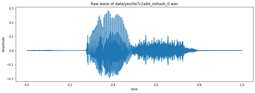
#Visualizing the audio - waveform
fig = plt.figure(figsize = (14,10))
ax1 = fig.add_subplot(211)
ax1.set_title('Raw wave of ' + 'data/yes/0a7c2a8d_nohash_0.wav')
ax1.set_xlabel('time')
ax1.set_ylabel('Amplitude')
ax1.plot(np.linspace(0, sample_rate/len(samples), sample_rate), samples)
#Visualizing the audio - waveform
import matplotlib.pyplot as plt
import librosa.display
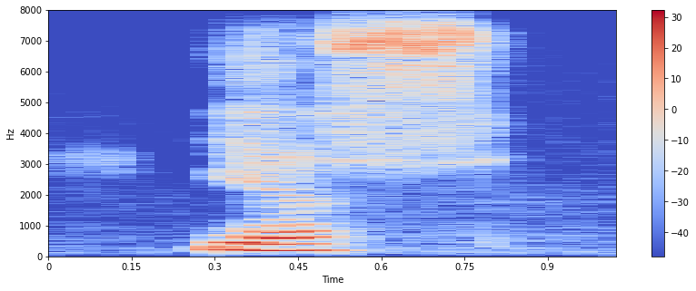
#Spectogram
samples_X = librosa.stft(samples)
Xdb = librosa.amplitude_to_db(abs(samples_X))
plt.figure(figsize=(14, 5))
librosa.display.specshow(Xdb, sr=sample_rate, x_axis='time', y_axis='hz')
plt.colorbar()
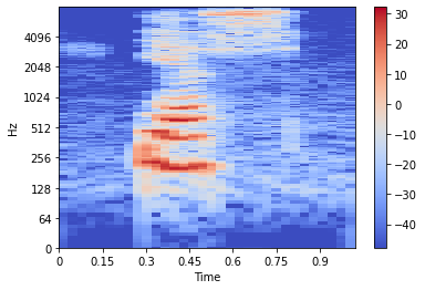
#Interchange the axis
librosa.display.specshow(Xdb, sr=sample_rate, x_axis='time', y_axis='log')
plt.colorbar()
Sampling rate
ipd.Audio(samples,rate = sample_rate)
print(sample_rate)
16000
Resampling
samples = librosa.resample(samples,sample_rate,8000)
ipd.Audio(samples,rate = 8000)
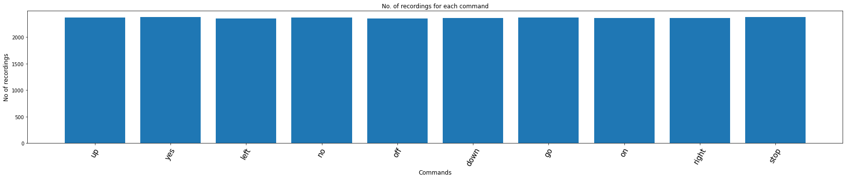
Number of recording of each voices
labels = os.listdir(train_audio_path)
labels
['up', 'yes', 'left', 'no', 'off', 'down', 'go', 'on', 'right', 'stop']
from matplotlib import cm
labels=os.listdir(train_audio_path)
#find count of each label and plot bar graph
no_of_recordings=[]
for label in labels:
    waves = [f for f in os.listdir(train_audio_path + label) if f.endswith('.wav')]
    no_of_recordings.append(len(waves))

#plot
plt.figure(figsize=(30,5))
index = np.arange(len(labels))
plt.bar(index, no_of_recordings)
plt.xlabel('Commands', fontsize=12)
plt.ylabel('No of recordings', fontsize=12)
plt.xticks(index, labels, fontsize=15, rotation=60)
plt.title('No. of recordings for each command')
plt.show()

labels=["yes", "no", "up", "down", "left", "right", "on", "off", "stop", "go"]
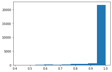
Duration of recordings
duration_of_recordings=[]
for label in labels:
    waves = [f for f in os.listdir(train_audio_path + '/'+ label) if f.endswith('.wav')]
    for wav in waves:
        sample_rate, samples = wavfile.read(train_audio_path + '/' + label + '/' + wav)
        duration_of_recordings.append(float(len(samples)/sample_rate))

plt.hist(np.array(duration_of_recordings))
Preprocessing the audio waves
from tqdm.notebook import tqdm # Notebook
#from tqdm import tqdm # Python
train_audio_path =DATASET_DIRECTORY_PATH+"/"
all_wave = []
all_label = []
for label in labels:
    print(label)
    waves = [f for f in os.listdir(train_audio_path + '/'+ label) if f.endswith('.wav')]
    #waves=waves[:20] # The first 20
    for wav in tqdm(waves):
        samples, sample_rate = librosa.load(train_audio_path + '/' + label + '/' + wav, sr = 16000)
        samples = librosa.resample(samples, sample_rate, 8000)
        if(len(samples)== 8000) :
            all_wave.append(samples)
            all_label.append(label)
from sklearn.preprocessing import LabelEncoder
le = LabelEncoder()
y = le.fit_transform(all_label)
classes = list(le.classes_)
len(all_wave)
21312
from keras.utils import np_utils
y = np_utils.to_categorical(y,num_classes = len(labels))
all_waves = np.array(all_wave).reshape(-1,8000,1)
Split into train and validation set
from sklearn.model_selection import train_test_split
#Extract training, test and validation datasets
#Split twice to get the validation set
x_tr, X_test, y_tr, y_test = train_test_split(np.array(all_wave), np.array(y), test_size=0.2, random_state=7, stratify=y)
x_tr, x_val, y_tr, y_val = train_test_split(x_tr, y_tr, test_size=0.2, random_state=7)
#Print the shapes
x_tr.shape, X_test.shape, x_val.shape, len(y_tr), len(y_test), len(y_val)
((13639, 8000), (4263, 8000), (3410, 8000), 13639, 4263, 3410)
Analisis of the Shape
#Print the shapes
x_tr.shape, y_tr.shape, len(y_tr)
((13639, 8000), (13639, 10), 13639)
index_col= 3 #index_of_column_you_need
print(y_tr[:,index_col])
[0. 0. 0. ... 0. 0. 0.]
print(len(y_tr[:,3]))
13639
Model - Conv Model for Speach Recognition

from keras.layers import Dense, Dropout, Flatten, Conv1D, Input, MaxPooling1D
from keras.models import Model
from keras.callbacks import EarlyStopping, ModelCheckpoint
from keras import backend as K
K.clear_session()

inputs = Input(shape=(8000,1))

#First Conv1D layer
conv = Conv1D(8,13, padding='valid', activation='relu', strides=1)(inputs)
conv = MaxPooling1D(3)(conv)
conv = Dropout(0.3)(conv)

#Second Conv1D layer
conv = Conv1D(16, 11, padding='valid', activation='relu', strides=1)(conv)
conv = MaxPooling1D(3)(conv)
conv = Dropout(0.3)(conv)

#Third Conv1D layer
conv = Conv1D(32, 9, padding='valid', activation='relu', strides=1)(conv)
conv = MaxPooling1D(3)(conv)
conv = Dropout(0.3)(conv)

#Fourth Conv1D layer
conv = Conv1D(64, 7, padding='valid', activation='relu', strides=1)(conv)
conv = MaxPooling1D(3)(conv)
conv = Dropout(0.3)(conv)

#Flatten layer
conv = Flatten()(conv)

#Dense Layer 1
conv = Dense(256, activation='relu')(conv)
conv = Dropout(0.3)(conv)

#Dense Layer 2
conv = Dense(128, activation='relu')(conv)
conv = Dropout(0.3)(conv)

outputs = Dense(len(labels), activation='softmax')(conv)

model = Model(inputs, outputs)
model.summary()
Model: "model"
_________________________________________________________________
 Layer (type)                Output Shape              Param #
=================================================================
 input_1 (InputLayer)        [(None, 8000, 1)]         0

 conv1d (Conv1D)             (None, 7988, 8)           112

 max_pooling1d (MaxPooling1D  (None, 2662, 8)          0
 )

 dropout (Dropout)           (None, 2662, 8)           0

 conv1d_1 (Conv1D)           (None, 2652, 16)          1424

 max_pooling1d_1 (MaxPooling  (None, 884, 16)          0
 1D)

 dropout_1 (Dropout)         (None, 884, 16)           0

 conv1d_2 (Conv1D)           (None, 876, 32)           4640

 max_pooling1d_2 (MaxPooling  (None, 292, 32)          0
 1D)

 dropout_2 (Dropout)         (None, 292, 32)           0

 conv1d_3 (Conv1D)           (None, 286, 64)           14400

 max_pooling1d_3 (MaxPooling  (None, 95, 64)           0
 1D)

 dropout_3 (Dropout)         (None, 95, 64)            0

 flatten (Flatten)           (None, 6080)              0

 dense (Dense)               (None, 256)               1556736

 dropout_4 (Dropout)         (None, 256)               0

 dense_1 (Dense)             (None, 128)               32896

 dropout_5 (Dropout)         (None, 128)               0

 dense_2 (Dense)             (None, 10)                1290

=================================================================
Total params: 1,611,498
Trainable params: 1,611,498
Non-trainable params: 0
_________________________________________________________________
model.compile(loss = 'categorical_crossentropy',optimizer = 'adam',metrics = ['accuracy'])
es = EarlyStopping(monitor = 'val_loss',mode = 'min',verbose = 1,patience = 10,min_delta = 0.0001)
mc = ModelCheckpoint('best_model.hdf5',monitor = 'val_acc',verbose = 1,save_best_only = True,mode = 'max')
history = model.fit(
    x_tr,
    y_tr,
    epochs = 100,
    callbacks=[es,mc],
    batch_size =32,
    validation_data = (x_val,y_val))
Epoch 1/100
427/427 [==============================] - ETA: 0s - loss: 2.0496 - accuracy: 0.2332
.
.
.
Epoch 32/100
425/427 [============================>.] - ETA: 0s - loss: 0.3039 - accuracy: 0.897
427/427 [==============================] - 4s 9ms/step - loss: 0.3041 - accuracy: 0.8971 - val_loss: 0.5104 - val_accuracy: 0.8419
Epoch 32: early stopping
model.save("best_model.hdf5")
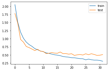
Diagnostic plot
from matplotlib import pyplot
pyplot.plot(history.history['loss'], label='train')
pyplot.plot(history.history['val_loss'], label='test')
pyplot.legend()
pyplot.savefig("plot.jpg")
pyplot.show()
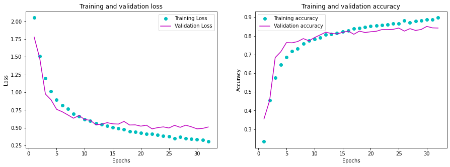
n_epochs = len(history.history['loss'])
early_epoch=n_epochs
#Adapted from Deep Learning with Python by Francois Chollet, 2018
history_dict=history.history
loss_values=history_dict['loss']
acc_values=history_dict['accuracy']
val_loss_values = history_dict['val_loss']
val_acc_values=history_dict['val_accuracy']
epochs=range(1,early_epoch+1)
fig,(ax1,ax2)=plt.subplots(1,2,figsize=(15,5))
ax1.plot(epochs,loss_values,'co',label='Training Loss')
ax1.plot(epochs,val_loss_values,'m', label='Validation Loss')
ax1.set_title('Training and validation loss')
ax1.set_xlabel('Epochs')
ax1.set_ylabel('Loss')
ax1.legend()
ax2.plot(epochs,acc_values,'co', label='Training accuracy')
ax2.plot(epochs,val_acc_values,'m',label='Validation accuracy')
ax2.set_title('Training and validation accuracy')
ax2.set_xlabel('Epochs')
ax2.set_ylabel('Accuracy')
ax2.legend()
plt.show()
Loading the best model
from keras.models import load_model
model=load_model('best_model.hdf5')
def predict(audio):
    prob=model.predict(audio.reshape(1,8000,1))
    index=np.argmax(prob[0])
    return classes[index]
import random
index=random.randint(0,len(x_val)-1)
print(index)
samples=x_val[index].ravel()
print("Audio:",classes[np.argmax(y_val[index])])
ipd.Audio(samples, rate=8000)
print("Text:",predict(samples))
140
Audio: off
Text: off
y_true_label = []
for  index in range(len(x_val)-1):
        y_true_label.append(classes[np.argmax(y_val[index])])
y_true = []
for  index in range(len(x_val)-1):
        y_true.append(np.argmax(y_val[index]))
test_labels = []
for  index in range(len(x_val)-1):
        test_labels.append(x_val[index].ravel())
y_pred_label = []
for i in test_labels:
    prediction=predict(i)
    y_pred_label.append(prediction)
y_pred = []
for audio in test_labels:
    prob=model.predict(audio.reshape(1,8000,1))
    prediction=np.argmax(prob[0])
    y_pred.append(prediction)
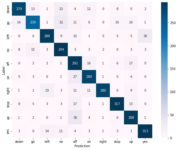
# Final evaluation of the model
scores = model.evaluate(x_val, y_val, verbose=0)
print("Accuracy: %.2f%%" % (scores[1]*100))
Accuracy: 84.19%
Predictions on the validation data:
import tensorflow as tf
import seaborn as sns
confusion_matrix = tf.math.confusion_matrix(y_true, y_pred)
plt.figure(figsize=(10, 8))
sns.heatmap(confusion_matrix, cmap="PuBu", robust=True,
            xticklabels=classes, yticklabels=classes,
            annot=True, fmt='g')
plt.xlabel('Prediction')
plt.ylabel('Label')
#plt.savefig(_PATH_TO_RESULTS+'/images/confusion_matrix.png')
Text(69.0, 0.5, 'Label')
You can download the notebook here or you can run it on Google Colab
![]()
Congratulations ! We have discussed and created a Neural Network to classify speech words by using CNN with Keras.
Leave a comment