Building Blocks of Neural Networks and TensorSpace

18 minute read

Hello, today I will discuss about the basic elements of the Neural Networks and have a picture of them.

When you are working in the developing of Machine Learning Models by using Neural Networks, and you have one particular problem, and you want to build a custom network for you particular problem and you don’t know how to start. Like happened to me he during the MMORPG-AI Network

One manner to learn new things is try to have a picture of the abstract thing and then describe it. I will introduce one interesting library that allows you visualize your custom neural network.

In addition I will try to introduce the building blocks of the Neural Networks in Keras that might help you to solve your problem.

For this project we need to install TensorSpace, this will us provide a fancy way to visualize some ideas beyond the Neural Networks.

Step 1 - Installation of Node.js

In a web browser, navigate to https://nodejs.org/en/download/. Click the Windows Installer button to download the latest default version. At the time this article was written, version 16.14.2 was the latest version. The Node.js installer includes the NPM package manager.

Open a command prompt (or PowerShell), and enter the following:

node -v

The system should display the Node.js version installed on your system. You can do the same for NPM:

npm -v

Microsoft Windows [Version 10.0.19044.1645]
(c) Microsoft Corporation. All rights reserved.

C:\Users\ruslamv>node -v
v16.14.2

C:\Users\ruslamv>npm -v
8.5.0

npm install --global yarn

Check that Yarn is installed by running:

yarn --version

C:\Users\ruslanmv>yarn --version
1.22.18

Step 2: Install TensorSpace

Install through NPM

npm install tensorspace

Step 3: Install TensorSpace converter

In ordering to use pretrained models we will use the TensorSpace Converter

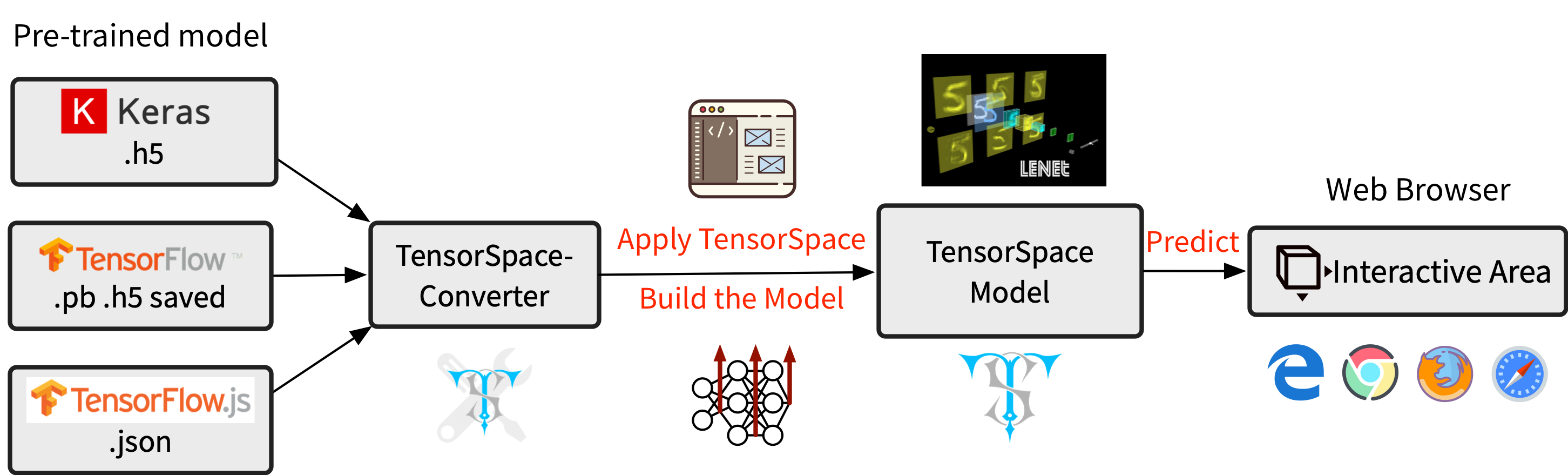
Unfortunatelly TensorSpace-Converter requires to run under Python 3.6, Node 11.3+, NPM 6.5+. If you have other pre-installed Python version in your local environment, we suggest you to create a new fresh virtual environment.

Let us install Anaconda here, after you have installed

conda create -n TensorSpace python=3.6
conda activate TensorSpace
pip install tensorspacejs keras

(pip install tensorflowjs)

If tensorspacejs is installed successfully, you can check the TensorSpace-Converter version by using the command:

$ tensorspacejs_converter -v

(TensorSpace36) C:\Users\project\tensorspacejs_converter -v 
Using TensorFlow backend.
tensorspacejs 0.2.0

Dependency versions:
python 3.6
node 11.3+
npm 6.5+
tensorflow 1.12.0
keras 2.2.2
tensorflowjs 0.8.0

tensorspacejs_converter --input_model_from="tensorflow"  --input_model_format="tf_keras" --output_layer_names="conv_1,maxpool_1,conv_2,maxpool_2,dense_1,dense_2,softmax" ./rawModel/keras/tf_keras_model.h5  ./saveModel/layerModel

After converting, we shall have the following preprocessed model:

(TensorSpace) C:\Users\project>tensorspacejs_converter --input_model_from="tensorflow"  --input_model_format="tf_keras" --output_layer_names="conv_1,maxpool_1,conv_2,maxpool_2,dense_1,dense_2,softmax" ./rawModel/keras/tf_keras_model.h5  ./saveModel/layerModel
Using TensorFlow backend.
2022-04-27 00:13:20.649887: I tensorflow/core/platform/cpu_feature_guard.cc:141] Your CPU supports instructions that this TensorFlow binary was not compiled to use: AVX2
Preprocessing hdf5 combined model...
Loading .h5 model into memory...
Generating multi-output encapsulated model...
Saving temp multi-output .h5 model...
Converting .h5 to web friendly format...
Using TensorFlow backend.
Deleting temp .h5 model...
Mission Complete!!!

(TensorSpace36) C:\Users\project>

Load and Visualize

First we need to download the libraries from here and include them into your html site

within

<script src="tf.min.js"></script>
<script src="three.min.js"></script>
<script src="Tween.min.js"></script>
<script src="TrackballControls.js"></script>
<script src="tensorspace.min.js"></script>

Then you should add the layer that you have generated

For layer model (tf.keras models) generated by TensorSpace-Converter:

model.load( {
    type: "tensorflow",
    url: "./saveModel/layerModel/model.json"
} );

If installed TensorSpace and preprocessed the pre-trained deep learning model successfully, let’s create an interactive 3D TensorSpace model.

First, we need to new a TensorSpace model instance:

let container = document.getElementById( "container" );
let model = new TSP.models.Sequential( container );

Next, based on the LeNet structure: Input + 2 X (Conv2D & Maxpooling) + 3 X (Dense), we build the structure of the model:

model.add( new TSP.layers.GreyscaleInput({ shape: [28, 28, 1] }) );
model.add( new TSP.layers.Padding2d({ padding: [2, 2] }) );
model.add( new TSP.layers.Conv2d({ kernelSize: 5, filters: 6, strides: 1 }) );
model.add( new TSP.layers.Pooling2d({ poolSize: [2, 2], strides: [2, 2] }) );
model.add( new TSP.layers.Conv2d({ kernelSize: 5, filters: 16, strides: 1 }) );
model.add( new TSP.layers.Pooling2d({ poolSize: [2, 2], strides: [2, 2] }) );
model.add( new TSP.layers.Dense({ units: 120 }) );
model.add( new TSP.layers.Dense({ units: 84 }) );
model.add( new TSP.layers.Output1d({
    units: 10,
    outputs: ["0", "1", "2", "3", "4", "5", "6", "7", "8", "9"]
}) );

Last, we should load the preprocessed TensorSpace compatible model and use init() method to create the TensorSpace model:

model.load({
    type: "tfjs",
    url: './lenetModel/mnist.json'
});
model.init(function(){
    console.log("Hello World from TensorSpace!");
});

We create our helloworld.html file

<!DOCTYPE html>
<html lang="en">
<head>
    <meta charset="UTF-8">
    <title>TensorSpace - Hello World</title>


    <script src="../lib/three.min.js"></script>
    <script src="../lib/tween.min.js"></script>
    <script src="../lib/tf.min.js"></script>
    <script src="../lib/TrackballControls.js"></script>
    <script src="../../dist/tensorspace.min.js"></script>

    <script src="../lib/jquery.min.js"></script>

    <style>

        html, body {
            margin: 0;
            padding: 0;
            width: 100%;
            height: 100%;
        }

        #container {
            width: 100%;
            height: 100%;
        }

    </style>

</head>
<body>

<div id="container"></div>

<script>

    $(function() {

		let modelContainer = document.getElementById( "container" );
		let model = new TSP.models.Sequential( modelContainer );

		model.add( new TSP.layers.GreyscaleInput() );
		model.add( new TSP.layers.Padding2d() );
		model.add( new TSP.layers.Conv2d() );
		model.add( new TSP.layers.Pooling2d() );
		model.add( new TSP.layers.Conv2d() );
		model.add( new TSP.layers.Pooling2d() );
		model.add( new TSP.layers.Dense() );
		model.add( new TSP.layers.Dense() );
		model.add( new TSP.layers.Output1d({
			outputs: ["0", "1", "2", "3", "4", "5", "6", "7", "8", "9"]
		}) );

		model.load({
			type: "tensorflow",
			url: './convertedModel/model.json'
		});
		model.init( function() {

			$.ajax({
				url: "./data/5.json",
				type: 'GET',
				async: true,
				dataType: 'json',
				success: function (data) {

					model.predict( data );

				}
			});


		} );

    });

</script>

</body>
</html>

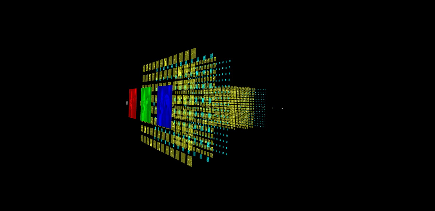
Then you can visualize like this

http://ruslanmv.com/assets/tensorspace/data/models/helloworld/helloworld.html

Fig 1 Example of Neural Network with Tensorspace

Let us discuss some of the building blocks of the Convolutional Neural Networks.

The convolutional layer in convolutional neural networks systematically applies filters to an input and creates output feature maps.

Stride

Stride is a parameter of the neural network’s filter that modifies the amount of movement over the image or video. Stride describes the process of increasing the step size by which you slide a filter over an input image. With a stride of 2, you advance the filter by two pixels at each step.

Same Padding

Same padding is the procedure of adding enough pixels at the edges so that the resulting feature map has the same dimensions as the input image to the convolution operation

same padding

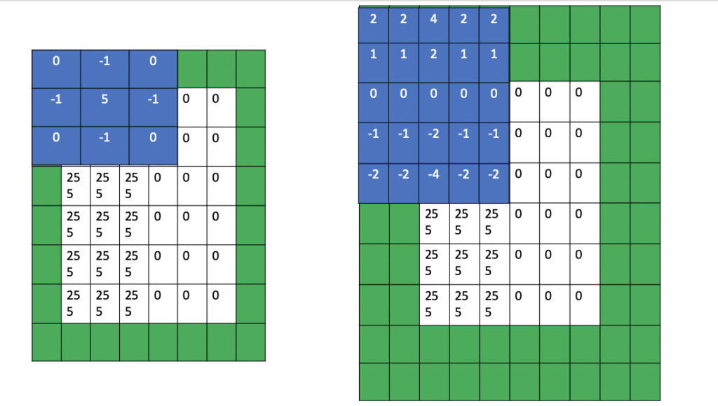
Fig 2 same padding for a 3×3 filter (left) and for a 5×5 filter (right)

Maxpooling

Formally, its function is to progressively reduce the spatial size of the representation to reduce the amount of parameters and computation in the network.

Max pooling is done to in part to help over-fitting by providing an abstracted form of the representation. As well, it reduces the computational cost by reducing the number of parameters to learn and provides basic translation invariance to the internal representation. Max pooling is done by applying a max filter to (usually) non-overlapping subregions of the initial representation.

Let’s say we have a 4x4 matrix representing our initial input. Let’s say, as well, that we have a 2x2 filter that we’ll run over our input. We’ll have a stride of 2 (meaning the (dx, dy) for stepping over our input will be (2, 2)) and won’t overlap regions.

For each of the regions represented by the filter, we will take the max of that region and create a new, output matrix where each element is the max of a region in the original input.

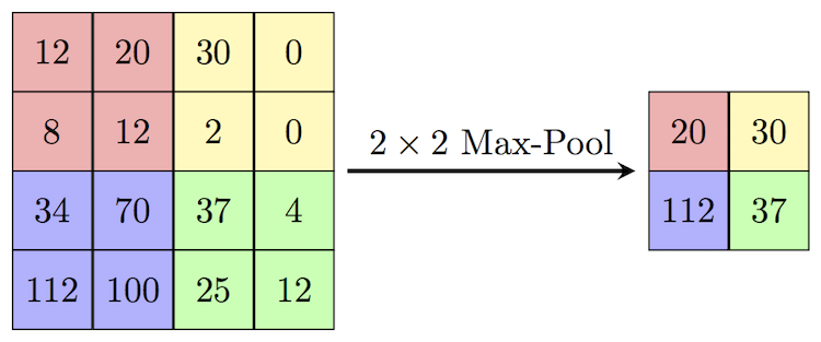
Fig 3 Pictorial representation

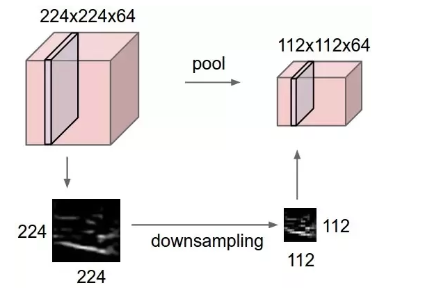
Fig 4 Real-life example

Building Blocks of the Neural Networks

There are 8 basic elements that I will consider to discuss:

Core Layers
Activation Layers
Convolution layers
Regularization layers
Pooling layers
Recurrent layers
Reshape layer
Flatten layer

1. Core Layers

Layers are the basic building blocks of neural networks in Keras. A layer consists of a tensor-in tensor-out computation function and some state, held in TensorFlow variables (the layer’s weights).

Input layer

The Input layer, is used to instantiate a Keras tensor. A Keras tensor is a symbolic tensor-like object, which we augment with certain attributes that allow us to build a Keras model just by knowing the inputs and outputs of the model.

Example

# this is a logistic regression in Keras
x = Input(shape=(32,))
y = Dense(16, activation='softmax')(x)
model = Model(x, y)

where the first arguments are:

shape: A shape tuple (integers), not including the batch size. For instance, shape=(32,) indicates that the expected input will be batches of 32-dimensional vectors.
batch_size: optional static batch size (integer).
name: An optional name string for the layer.

Dense layer

from tensorflow.keras import layers            
layer = layers.Dense(32, activation='relu')    
inputs = tf.random.uniform(shape=(10, 20))      
outputs = layer(inputs)                         

The dense layer is a neural network layer that is connected deeply, which means each neuron in the dense layer receives input from all neurons of its previous layer.

The Dense layer that implements the operation:

output = activation(dot(input, kernel) + bias)

where activation is the element-wise activation function passed as the activation argument, kernel is a weights matrix created by the layer, and bias is a bias vector created by the layer.

In other words,

Example

>>> # Create a `Sequential` model and add a Dense layer as the first layer.  
>>> model = tf.keras.models.Sequential()
>>> model.add(tf.keras.Input(shape=(16,)))
>>> model.add(tf.keras.layers.Dense(32, activation='relu'))
>>> # Now the model will take as input arrays of shape (None, 16)  
>>> # and output arrays of shape (None, 32).  
>>> # Note that after the first layer, you don't need to specify  
>>> # the size of the input anymore:  
>>> model.add(tf.keras.layers.Dense(32))
>>> model.output_shape
(None, 32)

The dense layer is found to be the most commonly used layer in the models. In the background, the dense layer performs a matrix-vector multiplication

If the input to the layer has a rank greater than 2, then Dense computes the dot product between the inputs and the kernel along the last axis of the inputs and axis 0 of the kernel

2. Activation Layers

An activation function in a neural network defines how the weighted sum of the input is transformed into an output from a node or nodes in a layer of the network

ReLu layer

The activations layer applies an activation function to an output for example ReLu

The rectified linear activation function or ReLU for short is a piecewise linear function that will output the input directly if it is positive, otherwise, it will output zero.

>>> layer = tf.keras.layers.ReLU()
>>> output = layer([-3.0, -1.0, 0.0, 2.0])
>>> list(output.numpy())
[0.0, 0.0, 0.0, 2.0]
>>> layer = tf.keras.layers.ReLU(max_value=1.0)
>>> output = layer([-3.0, -1.0, 0.0, 2.0])
>>> list(output.numpy())
[0.0, 0.0, 0.0, 1.0]

The rectified linear activation function overcomes the vanishing gradient problem, allowing models to learn faster and perform better

Sigmoid activation

Sigmoidal functions are frequently used in machine learning, specifically to model the output of a node or “neuron.” These functions are inherently non-linear and thus allow neural networks to find non-linear relationships between data features.

Sigmoid activation function, sigmoid(x) = 1 / (1 + exp(-x)).

For small values (<-5), sigmoid returns a value close to zero, and for large values (>5) the result of the function gets close to 1.

>>> a = tf.constant([-20, -1.0, 0.0, 1.0, 20], dtype = tf.float32)
>>> b = tf.keras.activations.sigmoid(a)
>>> b.numpy()
array([2.0611537e-09, 2.6894143e-01, 5.0000000e-01, 7.3105860e-01,
         1.0000000e+00], dtype=float32)

Softmax activation

The softmax function is used as the activation function in the output layer of neural network models that predict a multinomial probability distribution. That is, softmax is used as the activation function for multi-class classification problems where class membership is required on more than two class labels

The softmax of each vector x is computed as

exp(x) / tf.reduce_sum(exp(x)).

Softmax converts a vector of values to a probability distribution.

The elements of the output vector are in range (0, 1) and sum to 1.

Softmax is often used as the activation for the last layer of a classification network because the result could be interpreted as a probability distribution.

Tanh function

Tanh function is symmetric about the origin, where the inputs would be normalized and they are more likely to produce outputs (which are inputs to next layer)and also, they are on an average close to zero. … These are the main reasons why tanh is preferred and performs better than sigmoid (logistic).

Hyperbolic tangent activation function.

>>> a = tf.constant([-3.0,-1.0, 0.0,1.0,3.0], dtype = tf.float32)
>>> b = tf.keras.activations.tanh(a)
>>> b.numpy()
array([-0.9950547, -0.7615942,  0.,  0.7615942,  0.9950547], dtype=float32)

3. Convolution layers

1D convolution layer

1D Convolutional Neural Networks are used mainly used on text and 1D signals

This layer creates a convolution kernel that is convolved with the layer input over a single spatial (or temporal) dimension to produce a tensor of outputs. If use_bias is True, a bias vector is created and added to the outputs. Finally, if activation is not None, it is applied to the outputs as well.

>>> # The inputs are 128-length vectors with 10 timesteps, and the batch size  
>>> # is 4.  
>>> input_shape = (4, 10, 128)
>>> x = tf.random.normal(input_shape)
>>> y = tf.keras.layers.Conv1D(
... 32, 3, activation='relu',input_shape=input_shape[1:])(x)
>>> print(y.shape)
(4, 8, 32)

the firsts arguments are

filters: Integer, the dimensionality of the output space (i.e. the number of output filters in the convolution).
kernel_size: An integer or tuple/list of a single integer, specifying the length of the 1D convolution window.
strides: An integer or tuple/list of a single integer, specifying the stride length of the convolution. Specifying any stride value != 1 is incompatible with specifying any dilation_rate value != 1.
padding: One of "valid", "same" or "causal" (case-insensitive). "valid" means no padding. "same" results in padding with zeros evenly to the left/right or up/down of the input such that output has the same height/width dimension as the input. "causal" results in causal (dilated) convolutions, e.g. output[t] does not depend on input[t+1:]. Useful when modeling temporal data where the model should not violate the temporal order. See WaveNet: A Generative Model for Raw Audio, section 2.1.
activation: Activation function to use. If you don’t specify anything, no activation is applied ( see keras.activations).

Conv2D layer

2-D convolutional layer applies sliding convolutional filters to the input. The layer convolves the input by moving the filters along the input vertically and horizontally and computing the dot product of the weights and the input, and then adding a bias term.

2D convolution layer (e.g. spatial convolution over images).

This layer creates a convolution kernel that is convolved with the layer input to produce a tensor of outputs. If use_bias is True, a bias vector is created and added to the outputs. Finally, if activation is not None, it is applied to the outputs as well.

When using this layer as the first layer in a model, provide the keyword argument input_shape (tuple of integers or None, does not include the sample axis), e.g. input_shape=(128, 128, 3) for 128x128 RGB pictures in data_format="channels_last". You can use None when a dimension has variable size.

Examples

>>> # The inputs are 28x28 RGB images with `channels_last` and the batch   >>> # size is 4.   >>> input_shape = (4, 28, 28, 3) >>> x = tf.random.normal(input_shape) >>> y = tf.keras.layers.Conv2D( ... 2, 3, activation='relu', input_shape=input_shape[1:])(x) >>> print(y.shape) (4, 26, 26, 2)

Conv3D layer

A 3D Convolution is a type of convolution where the kernel slides in 3 dimensions as opposed to 2 dimensions with 2D convolutions. One example use case is medical imaging where a model is constructed using 3D image slices.

3D convolution layer (e.g. spatial convolution over volumes).

>>> # The inputs are 28x28x28 volumes with a single channel, and the  
>>> # batch size is 4  
>>> input_shape =(4, 28, 28, 28, 1)
>>> x = tf.random.normal(input_shape)
>>> y = tf.keras.layers.Conv3D(
... 2, 3, activation='relu', input_shape=input_shape[1:])(x)
>>> print(y.shape)
(4, 26, 26, 26, 2)

Conv2DTranspose layer

Conv2DTranspose is a convolution operation whose kernel is learnt (just like normal conv2d operation) while training your model. Using Conv2DTranspose will also upsample its input but the key difference is the model should learn what is the best upsampling for the job Transposed convolution layer (sometimes called Deconvolution).

The need for transposed convolutions generally arises from the desire to use a transformation going in the opposite direction of a normal convolution, i.e., from something that has the shape of the output of some convolution to something that has the shape of its input while maintaining a connectivity pattern that is compatible with said convolution.

new_rows = ((rows - 1) * strides[0] + kernel_size[0] - 2 * padding[0] +
output_padding[0])
new_cols = ((cols - 1) * strides[1] + kernel_size[1] - 2 * padding[1] +
output_padding[1])

Conv3DTranspose layer

Transposed convolution layer (sometimes called Deconvolution). The need for transposed convolutions generally arises from the desire to use a transformation going in the opposite direction of a normal convolution, i.e., from something that has the shape of the output of some convolution to something that has the shape of its input while maintaining a connectivity pattern that is compatible with said convolution.

4. Regularization layers

Dropout layer

Dropout is a technique used to prevent a model from overfitting. Dropout works by randomly setting the outgoing edges of hidden units (neurons that make up hidden layers) to 0 at each update of the training phase

Applies Dropout to the input.

The Dropout layer randomly sets input units to 0 with a frequency of rate at each step during training time, which helps prevent overfitting. Inputs not set to 0 are scaled up by 1/(1 - rate) such that the sum over all inputs is unchanged.

Note that the Dropout layer only applies when training is set to True such that no values are dropped during inference. When using model.fit, training will be appropriately set to True automatically, and in other contexts, you can set the kwarg explicitly to True when calling the layer.

>>> tf.random.set_seed(0)
>>> layer = tf.keras.layers.Dropout(.2, input_shape=(2,))
>>> data = np.arange(10).reshape(5, 2).astype(np.float32)
>>> print(data)
[[0. 1.]
 [2. 3.]
 [4. 5.]
 [6. 7.]
 [8. 9.]]
>>> outputs = layer(data, training=True)
>>> print(outputs)
tf.Tensor(
[[ 0.    1.25]
 [ 2.5   3.75]
 [ 5.    6.25]
 [ 7.5   8.75]
 [10.    0.  ]], shape=(5, 2), dtype=float32)

Layer weight regularizers

Regularizers allow you to apply penalties on layer parameters or layer activity during optimization. These penalties are summed into the loss function that the network optimizes.

Regularization penalties are applied on a per-layer basis. The exact API will depend on the layer, but many layers (e.g. Dense, Conv1D, Conv2D and Conv3D) have a unified AP

from tensorflow.keras import layers
from tensorflow.keras import regularizers

layer = layers.Dense(
    units=64,
    kernel_regularizer=regularizers.l1_l2(l1=1e-5, l2=1e-4),
    bias_regularizer=regularizers.l2(1e-4),
    activity_regularizer=regularizers.l2(1e-5)
)

5. Pooling layers

A pooling layer is a new layer added after the convolutional layer. Specifically, after a nonlinearity (e.g. ReLU) has been applied to the feature maps output by a convolutional layer; for example the layers in a model may look as follows: Input Image. Convolutional Layer

Maximum pooling, or max pooling, is a pooling operation that calculates the maximum, or largest, value in each patch of each feature map.

MaxPooling1D layer

Max pooling operation for 1D temporal data.

Max pooling operation for 1D temporal data. Downsamples the input representation by taking the maximum value over a spatial window of size pool_size . The window is shifted by strides .

Downsamples the input representation by taking the maximum value over a spatial window of size pool_size. The window is shifted by strides. The resulting output, when using the "valid" padding option, has a shape of: output_shape = (input_shape - pool_size + 1) / strides)

The resulting output shape when using the "same" padding option is: output_shape = input_shape / strides

>>> x = tf.constant([1., 2., 3., 4., 5.])
>>> x = tf.reshape(x, [1, 5, 1])
>>> max_pool_1d = tf.keras.layers.MaxPooling1D(pool_size=2,
...    strides=1, padding='valid')
>>> max_pool_1d(x)
<tf.Tensor: shape=(1, 4, 1), dtype=float32, numpy=
array([[[2.],
        [3.],
        [4.],
        [5.]]], dtype=float32)>

MaxPooling2D layer

Max pooling operation for 2D spatial data.

Downsamples the input along its spatial dimensions (height and width) by taking the maximum value over an input window (of size defined by pool_size) for each channel of the input. The window is shifted by strides along each dimension.

>>> x = tf.constant([[1., 2., 3.],
...                  [4., 5., 6.],
...                  [7., 8., 9.]])
>>> x = tf.reshape(x, [1, 3, 3, 1])
>>> max_pool_2d = tf.keras.layers.MaxPooling2D(pool_size=(2, 2),
...    strides=(1, 1), padding='valid')
>>> max_pool_2d(x)
<tf.Tensor: shape=(1, 2, 2, 1), dtype=float32, numpy=
  array([[[[5.],
           [6.]],
          [[8.],
           [9.]]]], dtype=float32)>

6. Recurrent layers

The RNN layer is comprised of a single rolled RNN cell that unrolls according to the “number of steps” value (number of time steps/segments) you provide. As we mentioned earlier the main speciality in RNNs is the ability to model short term dependencies. This is due to the hidden state in the RNN

LSTM layer

Long short-term memory (LSTM) is an artificial recurrent neural network (RNN) architecture used in the field of deep learning. Unlike standard feedforward neural networks, LSTM has feedback connections. … A common LSTM unit is composed of a cell, an input gate, an output gate and a forget gate.

Based on available runtime hardware and constraints, this layer will choose different implementations (cuDNN-based or pure-TensorFlow) to maximize the performance. If a GPU is available and all the arguments to the layer meet the requirement of the CuDNN kernel (see below for details), the layer will use a fast cuDNN implementation.

The requirements to use the cuDNN implementation are:

activation == tanh
recurrent_activation == sigmoid
recurrent_dropout == 0
unroll is False
use_bias is True
Inputs, if use masking, are strictly right-padded.
Eager execution is enabled in the outermost context.

>>> inputs = tf.random.normal([32, 10, 8])
>>> lstm = tf.keras.layers.LSTM(4)
>>> output = lstm(inputs)
>>> print(output.shape)
(32, 4)
>>> lstm = tf.keras.layers.LSTM(4, return_sequences=True, return_state=True)
>>> whole_seq_output, final_memory_state, final_carry_state = lstm(inputs)
>>> print(whole_seq_output.shape)
(32, 10, 4)
>>> print(final_memory_state.shape)
(32, 4)
>>> print(final_carry_state.shape)
(32, 4)

Gated Recurrent Unit - Cho et al. 2014.

See the Keras RNN API guide for details about the usage of RNN API.

The requirements to use the cuDNN implementation are:

activation == tanh
recurrent_activation == sigmoid
recurrent_dropout == 0
unroll is False
use_bias is True
reset_after is True
Inputs, if use masking, are strictly right-padded.
Eager execution is enabled in the outermost context.

>>> inputs = tf.random.normal([32, 10, 8])
>>> gru = tf.keras.layers.GRU(4)
>>> output = gru(inputs)
>>> print(output.shape)
(32, 4)
>>> gru = tf.keras.layers.GRU(4, return_sequences=True, return_state=True)
>>> whole_sequence_output, final_state = gru(inputs)
>>> print(whole_sequence_output.shape)
(32, 10, 4)
>>> print(final_state.shape)
(32, 4)

7. Reshape layer

The Reshape layer can be used to change the dimensions of its input, without changing its data. Just like the Flatten layer, only the dimensions are changed; no data is copied in the process. … Positive numbers are used directly, setting the corresponding dimension of the output blob.

`Reshape` class

tf.keras.layers.Reshape(target_shape, **kwargs)

Layer that reshapes inputs into the given shape.

Input shape

Arbitrary, although all dimensions in the input shape must be known/fixed. Use the keyword argument input_shape (tuple of integers, does not include the samples/batch size axis) when using this layer as the first layer in a model.

Output shape

(batch_size,) + target_shape

Example

>>> # as first layer in a Sequential model   >>> model = tf.keras.Sequential() >>> model.add(tf.keras.layers.Reshape((3, 4), input_shape=(12,))) >>> # model.output_shape == (None, 3, 4), `None` is the batch size.   >>> model.output_shape (None, 3, 4)

8. Flatten layer

Flatten is the function that converts the pooled feature map to a single column that is passed to the fully connected layer. Dense adds the fully connected layer to the neural network.

`Flatten` class

tf.keras.layers.Flatten(data_format=None, **kwargs)

Flattens the input. Does not affect the batch size.

Note: If inputs are shaped (batch,) without a feature axis, then flattening adds an extra channel dimension and output shape is (batch, 1).

Arguments

data_format: A string, one of channels_last (default) or channels_first. The ordering of the dimensions in the inputs. channels_last corresponds to inputs with shape (batch, ..., channels) while channels_first corresponds to inputs with shape (batch, channels, ...). It defaults to the image_data_format value found in your Keras config file at ~/.keras/keras.json. If you never set it, then it will be “channels_last”.

Example

>>> model = tf.keras.Sequential() >>> model.add(tf.keras.layers.Conv2D(64, 3, 3, input_shape=(3, 32, 32))) >>> model.output_shape (None, 1, 10, 64) 

>>> model.add(Flatten()) >>> model.output_shape (None, 640)

Models Examples

Now that we have seen some of the building blocks of the Neural Networks, we can visualize some of the neural networks.

If you are interested to download the papers or get more information about the previous models. You can visit this repository here.

References

https://tensorspace.org/

https://keras.io/

https://www.tensorflow.org/

https://keras.io/examples/

Congratulations! You have learned more about Neural Networks.

Share on

Twitter Facebook LinkedIn

Ruslan Magana Vsevolodovna

Step 1 - Installation of Node.js

Step 2: Install TensorSpace

Load and Visualize

Stride

Same Padding

Maxpooling

Building Blocks of the Neural Networks

1. Core Layers

Input layer

Dense layer

2. Activation Layers

ReLu layer

Sigmoid activation

Softmax activation

Tanh function

3. Convolution layers

1D convolution layer

Conv2D layer

Conv3D layer

Conv2DTranspose layer

Conv3DTranspose layer

4. Regularization layers

Dropout layer

Layer weight regularizers

5. Pooling layers

MaxPooling1D layer

MaxPooling2D layer

6. Recurrent layers

LSTM layer

7. Reshape layer

Reshape class

8. Flatten layer

Flatten class

Models Examples

References

Share on

Leave a comment

You may also enjoy

How to Fine Tune Mixtral-8x7B-Instruct model with PEFT in the Cloud

14 Apr 2024

Watsonx Assistant with Milvus as Vector Database

10 Mar 2024

How to Generate Images in Python with Diffusion Models

10 Feb 2024

How to create a React Application with IBM Carbon Design

31 Jan 2024

`Reshape` class

`Flatten` class