Regression with Neural Networks

For this project, we are going to work on evaluating price of houses given the following features:

1. Year of sale of the house
2. The age of the house at the time of sale
3. Distance from city center
4. Number of stores in the locality
5. The latitude
6. The longitude

Note: This notebook uses python 3 and these packages: tensorflow, pandas, matplotlib, scikit-learn.

Importing Libraries & Helper Functions

First of all, we will need to import some libraries and helper functions. This includes TensorFlow and some utility functions that I’ve written to save time.

import pandas as pd
import matplotlib.pyplot as plt
import tensorflow as tf

from utils import *
from sklearn.model_selection import train_test_split
from tensorflow.keras.models import Sequential
from tensorflow.keras.layers import Dense, Dropout
from tensorflow.keras.callbacks import EarlyStopping, LambdaCallback

%matplotlib inline
print('Libraries imported.')

Importing the Data

You can download the data from here.

The dataset is saved in a data.csv file. We will use pandas to take a look at some of the rows.

df = pd.read_csv('data.csv', names = column_names)
df.head()

Check Missing Data

It’s a good practice to check if the data has any missing values. In real world data, this is quite common and must be taken care of before any data pre-processing or model training.

df.isna()

	serial	date	age	distance	stores	latitude	longitude	price
0	False	False	False	False	False	False	False	False
1	False	False	False	False	False	False	False	False
2	False	False	False	False	False	False	False	False
3	False	False	False	False	False	False	False	False
4	False	False	False	False	False	False	False	False
...	...	...	...	...	...	...	...	...
4995	False	False	False	False	False	False	False	False
4996	False	False	False	False	False	False	False	False
4997	False	False	False	False	False	False	False	False
4998	False	False	False	False	False	False	False	False
4999	False	False	False	False	False	False	False	False

5000 rows × 8 columns

df.isna().sum()

serial       0
date         0
age          0
distance     0
stores       0
latitude     0
longitude    0
price        0
dtype: int64

We can see that there are no nun values

Data Normalization

We can make it easier for optimization algorithms to find minimas by normalizing the data before training a model.

df.head()

	serial	date	age	distance	stores	latitude	longitude	price
0	0	2009	21	9	6	84	121	14264
1	1	2007	4	2	3	86	121	12032
2	2	2016	18	3	7	90	120	13560
3	3	2002	13	2	2	80	128	12029
4	4	2014	25	5	8	81	122	14157

We will skip the first column serial, there are several ways to do, one is

df.iloc[:,1:].head()

	date	age	distance	stores	latitude	longitude	price
0	2009	21	9	6	84	121	14264
1	2007	4	2	3	86	121	12032
2	2016	18	3	7	90	120	13560
3	2002	13	2	2	80	128	12029
4	2014	25	5	8	81	122	14157

and we normalize

df = df.iloc[:,1:]
df_norm = (df - df.mean())/df.std()
df_norm.head()

	date	age	distance	stores	latitude	longitude	price
0	0.015978	0.181384	1.257002	0.345224	-0.307212	-1.260799	0.350088
1	-0.350485	-1.319118	-0.930610	-0.609312	0.325301	-1.260799	-1.836486
2	1.298598	-0.083410	-0.618094	0.663402	1.590328	-1.576456	-0.339584
3	-1.266643	-0.524735	-0.930610	-0.927491	-1.572238	0.948803	-1.839425
4	0.932135	0.534444	0.006938	0.981581	-1.255981	-0.945141	0.245266

Convert Label Value

Because we are using normalized values for the labels, we will get the predictions back from a trained model in the same distribution. So, we need to convert the predicted values back to the original distribution if we want predicted prices.

y_mean = df['price'].mean()
y_std = df['price'].std()

def convert_label_value(pred):
    return int(pred * y_std + y_mean)


print(convert_label_value(-1.836486), " that corresponds to the price 12032")

12031  that corresponds to the price 12032

Create Training and Test Sets

Select Features

Make sure to remove the column price from the list of features as it is the label and should not be used as a feature.

x = df_norm.iloc[:,:6]
x.head()

	date	age	distance	stores	latitude	longitude
0	0.015978	0.181384	1.257002	0.345224	-0.307212	-1.260799
1	-0.350485	-1.319118	-0.930610	-0.609312	0.325301	-1.260799
2	1.298598	-0.083410	-0.618094	0.663402	1.590328	-1.576456
3	-1.266643	-0.524735	-0.930610	-0.927491	-1.572238	0.948803
4	0.932135	0.534444	0.006938	0.981581	-1.255981	-0.945141

Select Labels

We select the prices

y = df_norm.iloc[:,-1:]
y.head()

	price
0	0.350088
1	-1.836486
2	-0.339584
3	-1.839425
4	0.245266

Feature and Label Values

We will need to extract just the numeric values for the features and labels as the TensorFlow model will expect just numeric values as input.

x_arr = x.values
y_arr = y.values

print('features array shape', x_arr.shape)
print('labels array shape', y_arr.shape)

features array shape (5000, 6)
labels array shape (5000, 1)

Train and Test Split

We will keep some part of the data aside as a test set. The model will not use this set during training and it will be used only for checking the performance of the model in trained and un-trained states. This way, we can make sure that we are going in the right direction with our model training.

x_train, x_test , y_train, y_test = train_test_split(x_arr,
                                                     y_arr, 
                                                     test_size = 0.05, 
                                                     random_state =0)
print( 'Training set', x_train.shape, y_train.shape)
print( 'Test set', x_test.shape, y_test.shape)

Training set (4750, 6) (4750, 1)
Test set (250, 6) (250, 1)

Let’s write a function that returns an untrained model of a certain architecture. We’re using a simple neural network architecture with just three hidden layers. We’re going to use the rail you activation function on all the layers except for the output layer.

Create the Model

We will use the sequential class from Keras. And the cool thing about this class is you can just pass on a list of layers to create your model architecture.

The first layer is a dense layer with just 10 nodes.

We know that input shape is simply a list of 6 values because we just have 6 features.

The activation is going to be really or rectified linear unit, and the next layer will be again a fully connected or dense layer.

And this time, let’s use 20 nodes and again, the same activation function relu and one more hidden layer with 5. nodes and finally, the output layer with just 1 node. so we have essentially, we have three hidden layers.

Create the Model

Let’s write a function that returns an untrained model of a certain architecture.

def get_model():
    model = Sequential([
        Dense(10, input_shape = (6,), activation = 'relu'),
        Dense(20, activation = 'relu'),
        Dense(5, activation = 'relu'),
        Dense(1) 
        
        
    ])
    
    model.compile(
         loss = 'mse',
         optimizer = 'adam'    
            )
    return model

This is the input and then we have three hidden layers. but 10, 20 and five nodes respectively. All the layers have activation function set to value except for the output layer. Since this is a regression problem, we just need the linear output without any activation function here.

These are all fully connected layers, and the number of parameters obviously correspond to the number of nodes that we have.

We need to specify a loss function in this case means great error, and we need to specify an optimizer.

In this case we are using Adam.

mse is a pretty common loss function used for regression problems. Remember This is the loss function that the optimization algorithm tries to minimize. And we are using a variant of stochastic gradient descent called Adam

An optimization algorithm is for and that is to minimize the loss of function.

get_model().summary()

Model: "sequential"
_________________________________________________________________
Layer (type)                 Output Shape              Param #   
=================================================================
dense (Dense)                (None, 10)                70        
_________________________________________________________________
dense_1 (Dense)              (None, 20)                220       
_________________________________________________________________
dense_2 (Dense)              (None, 5)                 105       
_________________________________________________________________
dense_3 (Dense)              (None, 1)                 6         
=================================================================
Total params: 401
Trainable params: 401
Non-trainable params: 0
_________________________________________________________________

The first dense layer that you see here is our first hidden there, which has 10 nodes.

The next one has 20 nodes. Next one has 5 nodes. And the final one node, the output there has one, and you can see that we have trainable parameters count 401.

Because these are dense layers, they are fully connected layers and if you want to understand how these parameters,count is arrived at, you can simply multiply the nodes in your output layer in in any one of these layers with the notes in the proceeding here.

So if you if you take a look at dense to for example, we have 5 nodes and in the preceding layer that is connected to we have 20 nodes, so each no disconnected.

Each node of dense one is connected to each note of dense two, which means we have total 100 connections. But you see that you have 105 parameters for the Slayer. Why is that? That’s simply because even though we have 100 weights, we also have a bias or intercept, in every layer.

Now that is just one interceptor connected to all the nodes of the layer that you calculating these parameters for so 520 gives you 100 and five into one gives you 5, and the total is 105 and you can do this exercise for all the layers and arrive at the same number of trainable parameters.

Model Training

We can use an EarlyStopping callback from Keras to stop the model training if the validation loss stops decreasing for a few epochs.

es_cb = EarlyStopping(monitor='val_loss',patience=5)
model = get_model()
preds_on_untrained = model.predict(x_test)
history = model.fit(
        x_train,y_train,
        validation_data =(x_test,y_test),
        epochs = 100,
        callbacks = [es_cb]

)

Epoch 1/100
149/149 [==============================] - 1s 3ms/step - loss: 0.6905 - val_loss: 0.2966
Epoch 2/100
149/149 [==============================] - 0s 1ms/step - loss: 0.2348 - val_loss: 0.1922
Epoch 3/100
149/149 [==============================] - 0s 1ms/step - loss: 0.1783 - val_loss: 0.1677
Epoch 4/100
149/149 [==============================] - 0s 1ms/step - loss: 0.1676 - val_loss: 0.1666
Epoch 5/100
149/149 [==============================] - 0s 1ms/step - loss: 0.1631 - val_loss: 0.1633
Epoch 6/100
149/149 [==============================] - 0s 1ms/step - loss: 0.1602 - val_loss: 0.1612
Epoch 7/100
149/149 [==============================] - 0s 1ms/step - loss: 0.1589 - val_loss: 0.1616
Epoch 8/100
149/149 [==============================] - 0s 1ms/step - loss: 0.1562 - val_loss: 0.1602
Epoch 9/100
149/149 [==============================] - 0s 1ms/step - loss: 0.1558 - val_loss: 0.1608
Epoch 10/100
149/149 [==============================] - 0s 1ms/step - loss: 0.1561 - val_loss: 0.1623
Epoch 11/100
149/149 [==============================] - 0s 2ms/step - loss: 0.1550 - val_loss: 0.1604
Epoch 12/100
149/149 [==============================] - 0s 1ms/step - loss: 0.1540 - val_loss: 0.1605
Epoch 13/100
149/149 [==============================] - 0s 2ms/step - loss: 0.1539 - val_loss: 0.1573
Epoch 14/100
149/149 [==============================] - 0s 1ms/step - loss: 0.1530 - val_loss: 0.1537
Epoch 15/100
149/149 [==============================] - 0s 1ms/step - loss: 0.1526 - val_loss: 0.1600
Epoch 16/100
149/149 [==============================] - 0s 1ms/step - loss: 0.1523 - val_loss: 0.1544
Epoch 17/100
149/149 [==============================] - 0s 1ms/step - loss: 0.1515 - val_loss: 0.1567
Epoch 18/100
149/149 [==============================] - 0s 1ms/step - loss: 0.1516 - val_loss: 0.1601
Epoch 19/100
149/149 [==============================] - 0s 1ms/step - loss: 0.1510 - val_loss: 0.1593

Plot Training and Validation Loss

Let’s use the plot_loss helper function to take a look training and validation loss.

plot_loss(history)

​
​

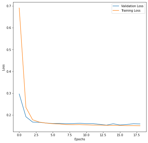
The training and validation loss. Values decreased as the training then don, and that’s great. But we don’t know yet if the train model actually makes reasonably accurate predictions. So let’s take a look at that. Now. Remember that we had some predictions on the untrained model. Similarly, we will make some predictions on the train model on the same data set, of course, which is X test.

Predictions

Plot Raw Predictions

Let’s use the compare_predictions helper function to compare predictions from the model when it was untrained and when it was trained.

preds_on_trained = model.predict(x_test)
compare_predictions(preds_on_untrained,preds_on_trained,y_test)

​
​

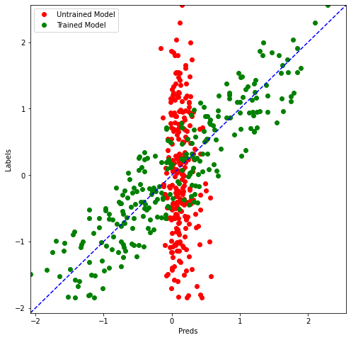
You can see the pattern. It’s pretty much a linear, uh, plot for the train model. Predictions now it’s making mistakes, of course, but the extent of those mistakes is, ah drastically less compared to what’s happening on the N train model. So, in an ideal situation, our model should make predictions same as labels. And that means this dotted blue line, right? But our green, uh, train model predictions are sort of following this started blue line, which means that our model training did actually work.

Plot Price Predictions

The plot for price predictions and raw predictions will look the same with just one difference: The x and y axis scale is changed.

price_untrained = [convert_label_value(y) for y in preds_on_untrained]
price_trained = [convert_label_value(y) for y in preds_on_trained]
price_test= [convert_label_value(y) for y in y_test]

compare_predictions(preds_on_untrained,preds_on_trained,y_test)

​
​

We pretty much get the same graph, but the ranges are now different. You can see the ranges from 12,000 to 16,000 or something for both predictions and labels You can see that the train model is a lot more aligned in its predictions to ground truth compared to the untrained model.

You can download the notebook here

Congratulations! we have created a neural network that performs regression.