
Forecast of Natural Gas Price with Deep Learning
Hello everyone today I am going to predict the Natural Gas Price using Time Series with Long short-term memory (LSTM) Neural Networks. This project can be used to predict any times series data. In this blog we are going to give you a Real Prediction of the Gas Price of the next week.
The financial data that we will use is investpy that is one of the most complete Python packages when it comes to financial data extraction to stop relying on public/private APIs since investpy is free and has no limitations. Is one good of financial data retrieval.
Step 1. Creation of the environment
Installation of Conda
First you need to install anaconda at this link

I will create an environment called forecast, but you can put the name that you like.
conda create -n forecast python==3.7
If you are running anaconda for first time, you should init conda with the shell that you want to work, in this case I choose the cmd.exe
conda init cmd.exe
and then close and open the terminal
conda activate forecast
then in your terminal type the following commands:
conda install ipykernel
python -m ipykernel install --user --name forecast --display-name "Python (Forecast)"
Then we install Tensorflow
pip install tensorflow==2.9.0
and Keras
pip install keras==2.9.0
If you will work with Forecasting projects I suggest install additional libraries:
pip install statsmodels pandas matplotlib sklearn plotly nbformat seaborn
We need to install investpy which allows the user to download both recent and historical data from all the financial products indexed at Investing.com.
we type
pip install investpy
Step 2 Download the Recent/Historical Data Retrieval
The following notebook details the process of training a neural network with LSTM models.
import numpy as np
import pandas as pd
from statsmodels.tsa.statespace.sarimax import SARIMAX
from statsmodels.graphics.tsaplots import plot_acf,plot_pacf
from statsmodels.tsa.seasonal import seasonal_decompose
import matplotlib.pyplot as plt
from sklearn.metrics import mean_squared_error
from statsmodels.tools.eval_measures import rmse
import warnings
warnings.filterwarnings("ignore")
import time
from datetime import date
from datetime import datetime
today = date.today()
print("Today's date:", today)
to_today = datetime.strptime(str(today), '%Y-%m-%d').strftime('%d/%m/%Y')
to_date = datetime.strptime(str(today), '%Y-%m-%d').strftime('%Y-%m-%d')
Today's date: 2022-07-11
def addonDays(a, x):
   ret = time.strftime("%Y-%m-%d",time.localtime(time.mktime(time.strptime(a,"%Y-%m-%d"))+x*3600*24+3600))
   return ret
week_ago=addonDays(to_date, -7)
week_ago
'2022-07-04'
Searching the Financial Data
The search function allows the user to tune the parameters to adjust the search results to their needs, where both product types and countries from where the products are, can be specified.
For this project we are looking for the price of Natural Gas but also can be used to predict prices of Crude Oil, Gold, Silver, Copper, etc.
In the text we write what we want to predict, in this project we use Natural Gas.
import investpy

gas_result = investpy.search_quotes(text='Natural Gas', products=['stocks'],
                                       countries=['united states'], n_results=1)
print(gas_result)
{"id_": 20413, "name": "Northwest Natural Gas Co", "symbol": "NWN", "country": "united states", "tag": "/equities/northwest-natural-gas-comp", "pair_type": "stocks", "exchange": "NYSE"}
Retrieved search results will be a list. those search results let the user retrieve both recent and historical data,
recent_data = gas_result.retrieve_recent_data()
print(recent_data.head())
             Open   High    Low  Close   Volume  Change Pct
Date
2022-06-13  53.31  53.56  51.28  51.51   214539       -4.77
2022-06-14  51.19  51.70  50.10  50.81   257471       -1.36
2022-06-15  50.94  51.63  50.51  50.81   337460        0.00
2022-06-16  50.28  51.01  49.69  50.86   428673        0.10
2022-06-17  51.43  51.99  50.56  51.69  1419987        1.63
Its information, the technical indicators, the default currency, etc., as presented in the piece of code below:
historical_data = gas_result.retrieve_historical_data(from_date='01/01/2022', to_date=to_today)
print(historical_data.head())
             Open   High    Low  Close  Volume  Change Pct
Date
2022-01-03  48.90  49.37  48.21  48.77  181573       -0.02
2022-01-04  49.10  49.79  49.08  49.35  131969        1.19
2022-01-05  49.47  49.89  49.24  49.57  126793        0.45
2022-01-06  49.72  49.74  49.27  49.54  130718       -0.06
2022-01-07  49.55  49.98  49.17  49.80  131915        0.52
information = gas_result.retrieve_information()
print(information)
{'prevClose': 52.06, 'dailyRange': '51.8-52.79', 'revenue': 894760000, 'open': 52.26, 'weekRange': '43.07-57.63', 'eps': 2.42, 'volume': 156807, 'marketCap': 1790000000, 'dividend': '1.93(3.71%)', 'avgVolume': 282206, 'ratio': 21.53, 'beta': 0.45, 'oneYearReturn': '0.12%', 'sharesOutstanding': 34255926, 'nextEarningDate': '11/08/2022'}
default_currency = gas_result.retrieve_currency()
print(default_currency)
USD
technical_indicators = gas_result.retrieve_technical_indicators(interval='daily')
print(technical_indicators)
              indicator           signal    value
0               RSI(14)          neutral  48.9150
1            STOCH(9,6)          neutral  45.0020
2          STOCHRSI(14)         oversold  19.5070
3           MACD(12,26)              buy   0.2100
4               ADX(14)          neutral  11.1960
5           Williams %R             sell -60.4200
6               CCI(14)          neutral -39.8620
7               ATR(14)  less_volatility   1.3331
8        Highs/Lows(14)          neutral   0.0000
9   Ultimate Oscillator              buy  51.6290
10                  ROC              buy   1.4510
11  Bull/Bear Power(13)             sell  -0.9120
import investpy

hist = investpy.get_stock_historical_data(stock='NWN',
                                        country='United States',
                                        from_date='01/01/2022',
                                        to_date=to_today)
print(hist.head())
             Open   High    Low  Close  Volume Currency
Date
2022-01-03  48.90  49.37  48.21  48.77  181573      USD
2022-01-04  49.10  49.79  49.08  49.35  131969      USD
2022-01-05  49.47  49.89  49.24  49.57  126793      USD
2022-01-06  49.72  49.74  49.27  49.54  130718      USD
2022-01-07  49.55  49.98  49.17  49.80  131915      USD
import plotly.graph_objects as go
fig = go.Figure(data=go.Scatter(x=hist.index,y=hist['Close'], mode='lines'))
fig.update_layout(title={'text':gas_result.name+' ('+ default_currency +')', 'x':0.5})
fig.show()
.png)
Drawing an indicator 20 Day Moving Average, pandas provides convenient ways to calculate time series-related metrics such as the moving average. The df.rolling() method provides “moving windows” that we can operate on. To get the average of the moving window, we just need to add the .mean() at the end of the rolling() method.
from plotly.subplots import make_subplots
fig2 = make_subplots(specs=[[{"secondary_y": True}]])
fig2.add_trace(go.Candlestick(x=hist.index,
                              open=hist['Open'],
                              high=hist['High'],
                              low=hist['Low'],
                              close=hist['Close'],
                             ))
fig2.add_trace(go.Scatter(x=hist.index,y=hist['Close'].rolling(window=20).mean(),marker_color='blue',name='20 Day MA'))
fig2.add_trace(go.Bar(x=hist.index, y=hist['Volume'], name='Volume'),secondary_y=True)
fig2.update_layout(title={'text':gas_result.name+' ('+ default_currency +')', 'x':0.5})
fig2.update_yaxes(range=[0,1000000000],secondary_y=True)
fig2.update_yaxes(visible=False, secondary_y=True)
fig2.update_layout(xaxis_rangeslider_visible=False)  #hide range slider
fig2.show()
.png)
Step 3 Creation of Dataframe
hist['Date'] = hist.index
df = hist[["Date", "Close"]]
df=df.reset_index(drop=True)
df.head()
| Date | Close | |
|---|---|---|
| 0 | 2022-01-03 | 48.77 |
| 1 | 2022-01-04 | 49.35 |
| 2 | 2022-01-05 | 49.57 |
| 3 | 2022-01-06 | 49.54 |
| 4 | 2022-01-07 | 49.80 |
df.info()
<class 'pandas.core.frame.DataFrame'>
RangeIndex: 130 entries, 0 to 129
Data columns (total 2 columns):
 #   Column  Non-Null Count  Dtype
---  ------  --------------  -----
 0   Date    130 non-null    datetime64[ns]
 1   Close   130 non-null    float64
dtypes: datetime64[ns](1), float64(1)
memory usage: 2.2 KB
df.Date = pd.to_datetime(df.Date)
df = df.set_index("Date")
df.head()
| Close | |
|---|---|
| Date | |
| 2022-01-03 | 48.77 |
| 2022-01-04 | 49.35 |
| 2022-01-05 | 49.57 |
| 2022-01-06 | 49.54 |
| 2022-01-07 | 49.80 |
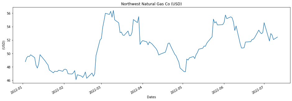
ax = df['Close'].plot(figsize = (16,5), title = gas_result.name+' ('+ default_currency +')')
ax.set(xlabel='Dates', ylabel=' ('+ default_currency +')');
This is the plot of the prices of the Natural Gas
Step 4 LSTM model training
Pre-processing data with MinMaxScaler
from sklearn.model_selection import train_test_split

train_data, test_data = train_test_split(df, test_size=0.2)
from sklearn.preprocessing import MinMaxScaler
scaler = MinMaxScaler()
scaler.fit(train_data)
scaled_train_data = scaler.transform(train_data)
scaled_test_data = scaler.transform(test_data)
Before creating the LSTM model, we need to create a Time Series Generator object.
from keras.preprocessing.sequence import TimeseriesGenerator
# Let's redefine to get 24 days  back and then predict the next day out
n_input = 24
n_features= 1
generator = TimeseriesGenerator(scaled_train_data, scaled_train_data,
                                length=n_input, batch_size=1)
Example of transformation
X,y = generator[0]
print(f'Given the Array: \n{X.flatten()}')
print(f'Predict this y: \n {y}')
Given the Array:
[0.31456311 0.52427184 0.36116505 0.25631068 0.2368932  0.79126214
 0.82427184 0.1368932  0.91067961 0.3592233  0.81941748 0.82330097
 0.52524272 0.6368932  1.         0.11747573 0.12135922 0.61553398
 0.70291262 0.14660194 0.54563107 0.20873786 0.90194175 0.08446602]
Predict this y:
 [[0.39223301]]
Long short-term memory (LSTM)
Long short-term memory is an artificial neural network used in the fields of artificial intelligence and deep learning. Unlike standard feedforward neural networks, LSTM has feedback connections. Such a recurrent neural network can process not only single data points, but also entire sequences of data.
We are going to present two models of LSTM, one with a Single LSTM contribution and with Double LSTM contribution.
Step 6 - Single LSTM Model
from keras.models import Sequential
from keras.layers import Dense
from keras.layers import LSTM
lstm_model = Sequential()
lstm_model.add(LSTM(50, activation='relu', input_shape=(n_input, n_features)))
lstm_model.add(Dense(1))
lstm_model.compile(optimizer='adam', loss='mse')
lstm_model.summary()
WARNING:tensorflow:Layer lstm will not use cuDNN kernels since it doesn't meet the criteria. It will use a generic GPU kernel as fallback when running on GPU.
Model: "sequential"
_________________________________________________________________
 Layer (type)                Output Shape              Param #
=================================================================
 lstm (LSTM)                 (None, 50)                10400

 dense (Dense)               (None, 1)                 51

=================================================================
Total params: 10,451
Trainable params: 10,451
Non-trainable params: 0
_________________________________________________________________
lstm_model.fit_generator(generator,epochs=20)
Epoch 1/20
80/80 [==============================] - 9s 97ms/step - loss: 0.1017
Epoch 2/20
.
.
.
80/80 [==============================] - 8s 96ms/step - loss: 0.0722
Epoch 20/20
80/80 [==============================] - 9s 107ms/step - loss: 0.0717

<keras.callbacks.History at 0x1bf63d0e518>
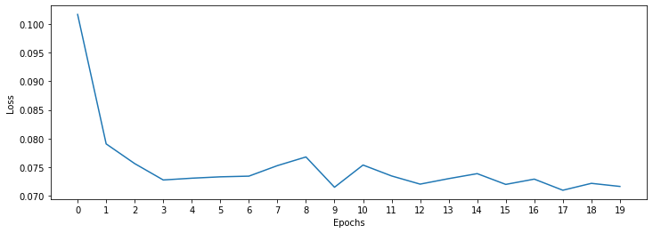
losses_lstm = lstm_model.history.history['loss']
plt.figure(figsize=(12,4))
plt.xlabel("Epochs")
plt.ylabel("Loss")
plt.xticks(np.arange(0,21,1))
plt.plot(range(len(losses_lstm)),losses_lstm);
Step 7 -Prediction on test data
Next we are going to make a prediction for 12 days (12 predictions). To do this we will do the following:
- create an empty list for each of our 12 predictions
- create the batch that our model will predict
- save the prediction in our list
- add the prediction to the end of the batch to use it in the next prediction
lstm_predictions_scaled = list()

batch = scaled_train_data[-n_input:]
current_batch = batch.reshape((1, n_input, n_features))

for i in range(len(test_data)):
    lstm_pred = lstm_model.predict(current_batch)[0]
    lstm_predictions_scaled.append(lstm_pred)
    current_batch = np.append(current_batch[:,1:,:],[[lstm_pred]],axis=1)
1/1 [==============================] - 0s 164ms/step
.
.
.
1/1 [==============================] - 0s 20ms/step
1/1 [==============================] - 0s 25ms/step
As you know, we scale our data, so we have to invert it to see true predictions.
lstm_predictions_scaled
[array([0.41446185], dtype=float32),
 array([0.4108159], dtype=float32),
.
.
.
 array([0.40563506], dtype=float32)]
lstm_predictions = scaler.inverse_transform(lstm_predictions_scaled)
lstm_predictions
array([[50.36895707],
       [50.33140371],
.
.
.
       [50.27945744],
       [50.27830387],
       [50.27804111]])
test_data['LSTM_Predictions'] = lstm_predictions
test_data['Close'].plot(figsize = (16,5), legend=True)
test_data['LSTM_Predictions'].plot(legend = True);
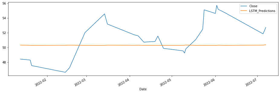
lstm_rmse_error = rmse(test_data['Close'], test_data["LSTM_Predictions"])
lstm_mse_error = lstm_rmse_error**2
mean_value = df['Close'].mean()

print(f'MSE Error: {lstm_mse_error}\nRMSE Error: {lstm_rmse_error}\nMean: {mean_value}')
MSE Error: 7.840908820950428
RMSE Error: 2.8001622847525156
Mean: 50.96569230769231
Step 6 -Double LSTM Model
from keras.models import Sequential
from keras.layers import Dense
from keras.layers import LSTM
from keras.callbacks import ModelCheckpoint
from keras.layers import Dropout

lstm_model = Sequential()
lstm_model.add(LSTM(200, activation='relu',return_sequences=True,
                    input_shape=(n_input, n_features)))
lstm_model.add(LSTM(200, return_sequences=True))
lstm_model.add(Dropout(rate=0.2))
lstm_model.add(LSTM(200, return_sequences=False))
lstm_model.add(Dense(1))

mc = ModelCheckpoint('double_model_lstm.h5', monitor='val_loss', mode='min',
                     verbose=1, save_best_only=True)

lstm_model.summary()
WARNING:tensorflow:Layer lstm_1 will not use cuDNN kernels since it doesn't meet the criteria. It will use a generic GPU kernel as fallback when running on GPU.
Model: "sequential_1"
_________________________________________________________________
 Layer (type)                Output Shape              Param #
=================================================================
 lstm_1 (LSTM)               (None, 24, 200)           161600

 lstm_2 (LSTM)               (None, 24, 200)           320800

 dropout (Dropout)           (None, 24, 200)           0

 lstm_3 (LSTM)               (None, 200)               320800

 dense_1 (Dense)             (None, 1)                 201

=================================================================
Total params: 803,401
Trainable params: 803,401
Non-trainable params: 0
_________________________________________________________________
lstm_model.compile(optimizer='adam', loss='mse')
lstm_model.fit_generator(generator,epochs=20)
Epoch 1/20
80/80 [==============================] - 14s 116ms/step - loss: 0.1063
Epoch 2/20
80/80 [==============================] - 10s 122ms/step - loss: 0.0803
Epoch 3/20
.
.
.
Epoch 19/20
80/80 [==============================] - 11s 133ms/step - loss: 0.0735
Epoch 20/20
80/80 [==============================] - 11s 139ms/step - loss: 0.0744

<keras.callbacks.History at 0x1bf6a9dae48>
Step 7 -EarlyStopping y Validation Generator
from tensorflow.keras.callbacks import EarlyStopping
early_stop = EarlyStopping(monitor='val_loss',
                           patience=12)
validation_generator = TimeseriesGenerator(scaled_test_data,scaled_test_data,
                                           length=n_input)
lstm_model.compile(optimizer='adam',
              loss='mse')
# fit model
lstm_model.fit_generator(generator,epochs=20,
                    validation_data=validation_generator,
                   callbacks=[early_stop, mc])
Epoch 1/20
80/80 [==============================] - ETA: 0s - loss: 0.0759
Epoch 1: val_loss improved from inf to 0.08796, saving model to double_model_lstm.h5
80/80 [==============================] - 15s 145ms/step - loss: 0.0759 - val_loss: 0.0880
Epoch 2/20
80/80 [==============================] - ETA: 0s - loss: 0.0773
.
.
.
Epoch 15/20
80/80 [==============================] - ETA: 0s - loss: 0.0694
Epoch 15: val_loss did not improve from 0.04324
80/80 [==============================] - 9s 117ms/step - loss: 0.0694 - val_loss: 0.2474

<keras.callbacks.History at 0x1bf6a830160>
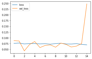
Learning curve
losses = pd.DataFrame(lstm_model.history.history)
losses.plot()
<AxesSubplot:>
from keras.models import load_model

lstm_model = load_model('double_model_lstm.h5', compile=False)
WARNING:tensorflow:Layer lstm_1 will not use cuDNN kernels since it doesn't meet the criteria. It will use a generic GPU kernel as fallback when running on GPU.
Step 8 -Prediction on test data
lstm_predictions_scaled = list()

batch = scaled_train_data[-n_input:]
current_batch = batch.reshape((1, n_input, n_features))

for i in range(len(test_data)):
    # get prediction 1 time stamp ahead ([0] is for grabbing just the number instead of [array])
    lstm_pred = lstm_model.predict(current_batch)[0]

    # store prediction
    lstm_predictions_scaled.append(lstm_pred)

    # update batch to now include prediction and drop first value
    current_batch = np.append(current_batch[:,1:,:],[[lstm_pred]],axis=1)
1/1 [==============================] - 1s 684ms/step
1/1 [==============================] - 0s 27ms/step
.
.
.
1/1 [==============================] - 0s 30ms/step
1/1 [==============================] - 0s 25ms/step
As you know, we scale our data, so we have to invert it to see true predictions.
Reverse the transformation
lstm_predictions = scaler.inverse_transform(lstm_predictions_scaled)
test_data['LSTM_Predictions'] = lstm_predictions
test_data['Close'].plot(figsize = (16,5), legend=True)
test_data['LSTM_Predictions'].plot(legend = True);

lstm_rmse_error = rmse(test_data['Close'], test_data["LSTM_Predictions"])
lstm_mse_error = lstm_rmse_error**2
mean_value = df['Close'].mean()

print(f'MSE Error: {lstm_mse_error}\nRMSE Error: {lstm_rmse_error}\nMean: {mean_value}')
MSE Error: 6.697523292919587
RMSE Error: 2.587957359177231
Mean: 50.96569230769231
Step 9 - Real Prediction of the Gas Price of the next week
Let us assume that we want to predict the price of the gas of the next week.
df.head()
| Close | |
|---|---|
| Date | |
| 2022-01-03 | 48.77 |
| 2022-01-04 | 49.35 |
| 2022-01-05 | 49.57 |
| 2022-01-06 | 49.54 |
| 2022-01-07 | 49.80 |
full_scaler = MinMaxScaler()
scaled_full_data = full_scaler.fit_transform(df)
length = 7 # Length of the output sequences (in number of timesteps)
generator = TimeseriesGenerator(scaled_full_data, scaled_full_data, length=length, batch_size=1)
model = Sequential()
model.add(LSTM(100, activation='relu', input_shape=(length, n_features)))
model.add(Dense(1))
model.compile(optimizer='adam', loss='mse')


# fit model
model.fit_generator(generator,epochs=8)
WARNING:tensorflow:Layer lstm_4 will not use cuDNN kernels since it doesn't meet the criteria. It will use a generic GPU kernel as fallback when running on GPU.
Epoch 1/8
123/123 [==============================] - 6s 43ms/step - loss: 0.0634
.
.
.
Epoch 8/8
123/123 [==============================] - 5s 39ms/step - loss: 0.0135

<keras.callbacks.History at 0x1c13b4f9b38>
forecast = []
# Replace periods with whatever forecast length you want
#one week
periods = 7

first_eval_batch = scaled_full_data[-length:]
current_batch = first_eval_batch.reshape((1, length, n_features))

for i in range(periods):

    # get prediction 1 time stamp ahead ([0] is for grabbing just the number instead of [array])
    current_pred = model.predict(current_batch)[0]

    # store prediction
    forecast.append(current_pred)

    # update batch to now include prediction and drop first value
    current_batch = np.append(current_batch[:,1:,:],[[current_pred]],axis=1)
1/1 [==============================] - 0s 140ms/step
1/1 [==============================] - 0s 21ms/step
1/1 [==============================] - 0s 17ms/step
1/1 [==============================] - 0s 17ms/step
1/1 [==============================] - 0s 23ms/step
1/1 [==============================] - 0s 19ms/step
1/1 [==============================] - 0s 18ms/step
forecast = scaler.inverse_transform(forecast)
test_data.tail()
| Close | LSTM_Predictions | |
|---|---|---|
| Date | ||
| 2022-01-21 | 47.54 | 51.572930 |
| 2022-04-21 | 51.55 | 51.572321 |
| 2022-06-08 | 54.70 | 51.570076 |
| 2022-03-14 | 54.56 | 51.570197 |
| 2022-05-18 | 51.07 | 51.569831 |
week_ago=addonDays(to_date, -7)
next_week=addonDays(to_date, 7)
next_month=addonDays(to_date, 30)
forecast_index = pd.date_range(start=to_date,periods=periods,freq='D')
forecast_index
DatetimeIndex(['2022-07-11', '2022-07-12', '2022-07-13', '2022-07-14',
               '2022-07-15', '2022-07-16', '2022-07-17'],
              dtype='datetime64[ns]', freq='D')
forecast_df = pd.DataFrame(data=forecast,index=forecast_index,
                           columns=['Forecast'])
forecast_df
| Forecast | |
|---|---|
| 2022-07-11 | 52.077826 |
| 2022-07-12 | 51.977773 |
| 2022-07-13 | 51.993099 |
| 2022-07-14 | 51.897952 |
| 2022-07-15 | 51.862930 |
| 2022-07-16 | 51.860414 |
| 2022-07-17 | 51.833954 |
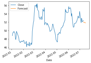
ax = df.plot()
forecast_df.plot(ax=ax)
<AxesSubplot:xlabel='Date'>
month_ago=addonDays(to_date, -30)
ax = df.plot()
forecast_df.plot(ax=ax)
plt.xlim(month_ago,next_week)
(19154.0, 19191.0)
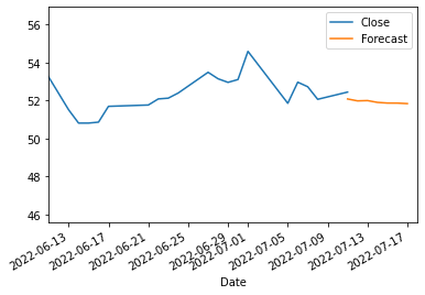
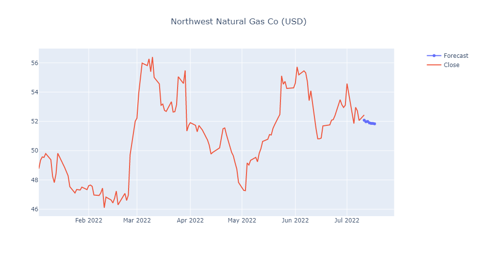
fig3 = make_subplots(specs=[[{"secondary_y": True}]])
fig3.add_trace(go.Scatter(x=forecast_df.index,y=forecast_df['Forecast'],name='Forecast'))
fig3.add_trace(go.Scatter(x=df.index,y=df['Close'],name='Close'))
fig3.update_layout(title={'text':gas_result.name+' ('+ default_currency +')', 'x':0.5})
fig3.update_yaxes(range=[0,1000000000],secondary_y=True)
fig3.update_yaxes(visible=False, secondary_y=True)
fig3.update_layout(xaxis_rangeslider_visible=False)  #hide range slider
fig3.show()
You can download the notebook here or you can run it on Google Colab ![]() .
.
Congratulations! We have created a Neural Network by using LSTM and we have predict the Natural Gas for one week.
Leave a comment