Twitter Sentiment Analysis by Geographical Area

Hello, today we are going to perform a Twitter Sentiment Analysis by a custom Geographical Area. In this blog post we are not use the Twitter Developer Account, instead I will use a simple and unlimited Twitter scraper with python.

I am interested to get top tweets with a custom keyword , geolocated less than 50 km from White House in the United States. I would like to analyze the word “gas” around the White House during one month since the February 24 2022 .

​ White House in United States

Installation of Conda

First you need to install anaconda at this link

in this location C:\Anaconda3 , then you, check that your terminal , recognize conda

C:\conda --version
conda 4.12.0

Step 1. Environment creation

The environments supported that I will consider is Python 3.7,

I will create an environment called twitter, but you can put the name that you like.

conda create -n twitter python==3.7

then we activate

conda activate twitter

then in your terminal type the following commands:

conda install ipykernel

then

python -m ipykernel install --user --name twitter --display-name "Python (Twitter)"

you will get something like

(twitter) C:\Users\ruslamv>python -m ipykernel install --user --name twitter --display-name "Python (Twitter)"
Installed kernelspec twitter in C:\Users\ruslanmv\AppData\Roaming\jupyter\kernels\twitter

If you want to delete your conda environment

conda env remove -n twitter

Step 2. Installation of the repositories

pip install certifi pandas python-dotenv chromedriver-autoinstaller geckodriver-autoinstaller urllib3 seaborn sklearn

pip install selenium==4.2.0 

and finally the great scrapper

pip install Scweet==1.8

and the geolocation

pip install geopy

and to analize the text

pip install wordcloud nltk

then open the Jupyter notebook with the command

jupyter notebook&

Let us get top tweets with a custom keyword like ‘gas’ geolocated less than 50 km from White house.

In this notebook we are going to classify important and no important twitter text messages by considering the number of likes. We are going to webscrap one month of twitter messages and analize them. We will choose one geographical area and from it , we will consider a radio around it and extract all possible twitts that contains a keyword of your interest.

For this blogpost we will consider the keyword gas and we will choose the White House and we are going to choose the dates one month after the War In Ukraine started. Just for curiosity. Get started. The interesting thing is that we do not need any account with twitter and the requests are unlimited and free.

Step 3. Getting the data

After the notebook is open you can import and use the functions as follows:

#Loading Libraries

from Scweet.scweet import scrape
from Scweet.user import get_user_information, get_users_following, get_users_followers
from geopy.geocoders import Nominatim

The first step is initialize the geolocator engine

geolocator = Nominatim(user_agent="twitter")

Selection of place

Here we need to specify the address you want to perform the analysis , for example, you can choose your home address or the street and number that you want to perform the research, in my case I chose the White House.

location = geolocator.geocode(" White House ") 

print(location.address)

White House, 1600, Pennsylvania Avenue Northwest, Washington, District of Columbia, 20500, United States

print((location.latitude, location.longitude))

(38.897699700000004, -77.03655315)

and we setup the radius that we want to explorer

distance="50km"

geolocation=str(location.latitude)+","+str(location.longitude)+","+str(distance)

geolocation

'38.897699700000004,-77.03655315,50km'

and also the period of time that you want to perform the research, then we create the dataset as follows, after this, we will wait a while until the webscrapping will work, and extract all the data

data = scrape(words=['gas'],
              since="2022-02-24", 
              until="2022-03-24", 
              from_account = None,      
              interval=1, 
              headless=False, 
              display_type="Top", 
              save_images=False, lang="en",
              resume=False, 
              filter_replies=False,
              proximity=False,
              geocode=geolocation)

looking for tweets between 2022-02-24 and 2022-02-25 ...
.
.
.

you can see the shape

data.shape

(420, 11)

you can save the data

data.to_csv('my_twitter.csv', index=False)

Get the main information of a given list of users. From the data, you can identify one single user

users = ['BrianJohnsonMPA',] 

# this function return a list that contains : 
# ["nb of following","nb of followers", "join date", "birthdate", "location", "website", "description"]
users_info = get_user_information(users, headless=True)

Scraping on headless mode.
--------------- BrianJohnsonMPA information : ---------------
Following :  3,370
Followers :  1,067
Location :  Washington, DC
Join date :  Joined July 2015
Birth date :  
Description :  VP Gov & Public Affairs / Head of Office, Veterans Guardian | Past: Vogel Group, American Petroleum Institute & Americans for Tax Reform | views my own
Website :  https://t.co/SXSxU0WBXH

as you see you can get a lot of information that can be very useful to the analysis of the region.

Moreover you can extract more information of the single user.

import pandas as pd

users_df = pd.DataFrame(users_info, index = ["nb of following","nb of followers", "join date", 
                                             "birthdate", "location", "website", "description"]).T
users_df

	nb of following	nb of followers	join date	birthdate	location	website	description
BrianJohnsonMPA	3,370	1,067	Joined July 2015		Washington, DC	https://t.co/SXSxU0WBXH	VP Gov & Public Affairs / Head of Office, Vete...

Interesting, well, let us continue to clean our dataset.

import pandas as pd
import numpy as np
import seaborn as sns
import matplotlib.pyplot as plt

df=pd.read_csv('my_twitter.csv') 

We replace NAN values with 0 ror the whole DataFrame using pandas

df=df.fillna(0)

df.head()

	UserScreenName	UserName	Timestamp	Text	Embedded_text	Emojis	Comments	Likes	Retweets	Image link	Tweet URL
0	Tommie Collins	@tommiecollins	2022-02-24T01:30:26.000Z	Tommie Collins\n@tommiecollins\n·\nFeb 24	So hold up...gas is almost $4 and y'all drivin...	0	6.0	22.0	68	['https://pbs.twimg.com/ext_tw_video_thumb/149...	https://twitter.com/tommiecollins/status/14966...
1	David Nichols	@DavidNichols_31	2022-02-24T22:15:45.000Z	David Nichols\n@DavidNichols_31\n·\nFeb 24	My only take on the War in the Ukraine is I be...	0	0.0	1.0	4	[]	https://twitter.com/DavidNichols_31/status/149...
2	KratosOfPortugal	@KratosPRT	2022-02-24T03:35:14.000Z	KratosOfPortugal\n@KratosPRT\n·\nFeb 24	Get ready for expensive gas.\nAFP News Agency\...	0	0.0	0.0	7	['https://pbs.twimg.com/profile_images/1272776...	https://twitter.com/KratosPRT/status/149669015...
3	Samuel Hammond	@hamandcheese	2022-02-24T17:26:52.000Z	Samuel Hammond\n@hamandcheese\n·\nFeb 24	Atlantic Canada is sitting on trillions of cub...	🌐 🏛 🏗	2.0	5.0	34	['https://pbs.twimg.com/profile_images/1437631...	https://twitter.com/hamandcheese/status/149689...
4	Brian M. Johnson MPA	@BrianJohnsonMPA	2022-02-24T19:06:04.000Z	Brian M. Johnson MPA\n@BrianJohnsonMPA\n·\nFeb 24	Replying to \n@JerryDunleavy\nOil & natural ga...	0	3.0	3.0	16	[]	https://twitter.com/BrianJohnsonMPA/status/149...

and let us choose the information that it is more relevant for us

dfa=df[['Embedded_text','Likes','Comments','Retweets','UserName']]

dfa.head()

	Embedded_text	Likes	Comments	Retweets	UserName
0	So hold up...gas is almost $4 and y'all drivin...	22.0	6.0	68	@tommiecollins
1	My only take on the War in the Ukraine is I be...	1.0	0.0	4	@DavidNichols_31
2	Get ready for expensive gas.\nAFP News Agency\...	0.0	0.0	7	@KratosPRT
3	Atlantic Canada is sitting on trillions of cub...	5.0	2.0	34	@hamandcheese
4	Replying to \n@JerryDunleavy\nOil & natural ga...	3.0	3.0	16	@BrianJohnsonMPA

df = dfa.sort_values(by=['Likes','Retweets','Comments'], ascending=False)

df.head(10)

	Embedded_text	Likes	Comments	Retweets	UserName
378	It doesn’t matter what a gallon of gas costs-r...	473.0	58.0	2,739	@JJCarafano
323	"We're banning all imports of Russian gas, oil...	424.0	70.0	2,316	@Liveuamap
185	These are also known as “pump gas with ya gloc...	109.0	7.0	109	@_JuiceJones
322	Gas is already at $4.33 a gallon here in DC, i...	93.0	187.0	575	@IntelDoge
219	In the search for new measures against becaus...	80.0	24.0	534	@carlbildt
377	Good piece. I’ll add that i saw a thread yeste...	55.0	10.0	199	@SaysSimonson
47	Seeing whole columns of Russian armor out of g...	43.0	9.0	249	@klonkitchen
396	The EU spent almost 13 million EUR on Russian ...	41.0	5.0	88	@SashaUstinovaUA
151	Multiple sources tell me investigators believe...	40.0	3.0	16	@Brad7News
375	Gas might 5+ but riding dick is freee shordy\n...	38.0	3.0	98	@nikkotank

We have created a single dataset of messages around the white house.

Step 4. Creation of the dataset

We are interested to classify the twitter messages by the importance or relevance,

• Imporant
• Unimportant

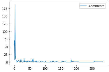
df=df.reset_index(drop=True)

df.plot(y='Likes', use_index=True)

# selecting rows based on condition
df_likes = df.loc[df['Likes'] != 0]
df_likes.shape

(116, 5)

# selecting rows based on condition
df_retweets = df.loc[df['Retweets'] != 0]
df_retweets.shape

(253, 5)

# selecting rows based on condition
df_comments = df.loc[df['Comments'] != 0]
df_comments.shape

(161, 5)

Step 5. Labelling the messages

In this part, we will consider the unimportant messages, that there are not likes, neither retweets or comments.

df_unimportant=df.loc[(df['Likes'] == 0) & (df['Retweets'] == 0)&(df['Comments'] == 0)]
df_unimportant.shape

(135, 5)

and the important messages with likes, retweets and comments,

df_important=df.loc[(df['Likes'] != 0) | (df['Retweets'] != 0)|(df['Comments'] != 0)]
df_important.shape

(285, 5)

# We check if our dimensions are okay
assert df_important.shape[0] +df_unimportant.shape[0] == df.shape[0], 'something is wrong'
print('its okay, the number of total messages are:',df.shape[0])

its okay, the number of total messages are: 420

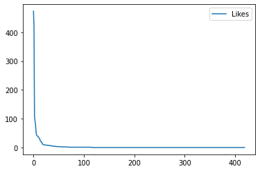
df_important=df_important.reset_index(drop=True)

df_important.plot(y='Comments', use_index=True)

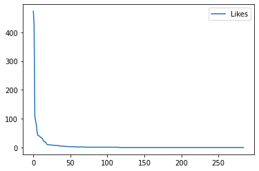
df_important.plot(y='Likes', use_index=True)

​
​

If we split the set of important twits into 3 categories we can do this approach

size=int(len(df_important)/3)

size

95

It is possible split the the importance of the message may be splitted in

1. Very Important
2. Fairly Important
3. Slightlly important
4. Not at all important

s# splitting dataframe by row index
df_1 = df_important.iloc[:size,:]
df_2 = df_important.iloc[size:2*size,:]
df_3 = df_important.iloc[2*size:s,:]
df_4 = df_unimportant

However we are dealing with very few messages we cannot proceed with this approach, if you have larger dataset for sure you can proceed this way.

df_1.head()

	Embedded_text	Likes	Comments	Retweets	UserName
0	It doesn’t matter what a gallon of gas costs-r...	473.0	58.0	2,739	@JJCarafano
1	"We're banning all imports of Russian gas, oil...	424.0	70.0	2,316	@Liveuamap
2	These are also known as “pump gas with ya gloc...	109.0	7.0	109	@_JuiceJones
3	Gas is already at $4.33 a gallon here in DC, i...	93.0	187.0	575	@IntelDoge
4	In the search for new measures against becaus...	80.0	24.0	534	@carlbildt

print("Shape of new dataframes - {} , {}, {}".format(df_1.shape, df_2.shape,df_3.shape))

Shape of new dataframes - (95, 5) , (95, 5), (95, 5)

# Create a sample dataframe with an text index
plotdata = pd.DataFrame(
    {"Twitter Classes": [len(df_1), len(df_2), len(df_3), len(df_4)]}, 
    index=["Very Important", 
           "Fairly Important", 
           "Slightlly important", 
           "Not at all important"])
# Plot a bar chart
plotdata.plot(kind="bar")

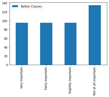
but for simplicity we choose only two types, important and not important messages.

Step 6. Let us consider only two classes important and not important

df_1['label'] = 0
df_2['label'] = 0
df_3['label'] = 1
df_4['label'] = 1

	Embedded_text	Likes	Comments	Retweets	UserName	label
190	Replying to \n@janjowen\nWhat if I want to rem...	0.0	2.0	1	@mls1776	1
191	Replying to \n@schlthss\nEven our EVs depend o...	0.0	1.0	1	@sogand_karbalai	1
192	Replying to \n@baecariss\nAll gas no break! \n...	0.0	1.0	1	@Team_Newby1	1
193	Replying to \n@tharealcatmom\nCramps and gas. ...	0.0	1.0	1	@itstifftiara	1
194	Replying to \n@Jim__840\n and \n@Arriadna\nThi...	0.0	1.0	1	@sonofnels	1

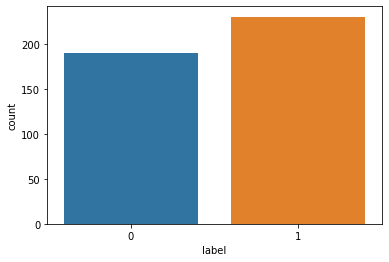
There is slightlly unbalanced data

# concatenating df1 and df2 along rows
df_twitter = pd.concat([df_1, df_2,df_3,df_4], axis=0)

df_twitter.rename(columns = {'Embedded_text':'tweet'}, inplace = True)

df_twitter.to_csv('twitter_gas.csv', index=False)

# Load the data
tweets_df = pd.read_csv('twitter_gas.csv')

tweets_df.shape

(420, 6)

tweets_df.head()

	tweet	Likes	Comments	Retweets	UserName	label
0	It doesn’t matter what a gallon of gas costs-r...	473.0	58.0	2,739	@JJCarafano	0
1	"We're banning all imports of Russian gas, oil...	424.0	70.0	2,316	@Liveuamap	0
2	These are also known as “pump gas with ya gloc...	109.0	7.0	109	@_JuiceJones	0
3	Gas is already at $4.33 a gallon here in DC, i...	93.0	187.0	575	@IntelDoge	0
4	In the search for new measures against becaus...	80.0	24.0	534	@carlbildt	0

tweets_df.info()

<class 'pandas.core.frame.DataFrame'>
RangeIndex: 420 entries, 0 to 419
Data columns (total 6 columns):
 #   Column    Non-Null Count  Dtype  
---  ------    --------------  -----  
 0   tweet     420 non-null    object 
 1   Likes     420 non-null    float64
 2   Comments  420 non-null    float64
 3   Retweets  420 non-null    object 
 4   UserName  420 non-null    object 
 5   label     420 non-null    int64  
dtypes: float64(2), int64(1), object(3)
memory usage: 19.8+ KB

# Drop the 'id' column
tweets_df = tweets_df.drop(['Likes', 'Comments', 'Retweets', 'UserName'], axis=1)

tweets_df.head()

	tweet	label
0	It doesn’t matter what a gallon of gas costs-r...	0
1	"We're banning all imports of Russian gas, oil...	0
2	These are also known as “pump gas with ya gloc...	0
3	Gas is already at $4.33 a gallon here in DC, i...	0
4	In the search for new measures against becaus...	0

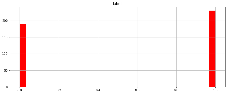
tweets_df.hist(bins = 30, figsize = (13,5), color = 'r')

sns.countplot(tweets_df['label'], label = "Count")

# Let's get the length of the messages
tweets_df['length'] = tweets_df['tweet'].apply(len)

tweets_df.head()

	tweet	label	length
0	It doesn’t matter what a gallon of gas costs-r...	0	131
1	"We're banning all imports of Russian gas, oil...	0	197
2	These are also known as “pump gas with ya gloc...	0	67
3	Gas is already at $4.33 a gallon here in DC, i...	0	125
4	In the search for new measures against becaus...	0	284

tweets_df.describe()

	label	length
count	420.000000	420.000000
mean	0.547619	178.990476
std	0.498321	116.781234
min	0.000000	20.000000
25%	0.000000	93.750000
50%	1.000000	148.500000
75%	1.000000	258.000000
max	1.000000	677.000000

# Let's see the shortest message 
tweets_df[tweets_df['length'] == 20]['tweet'].iloc[0]

'Premium gas is 5.30?'

# Let's view the message with mean length 
tweets_df[tweets_df['length'] == 178]['tweet'].iloc[0]

'The EU spent almost 13 million EUR on Russian coal, oil, and gas since the Kremlin’s war on Ukraine began on February 24. \n\nStop financing Putin’s war machine! #StopPutin\n5\n41\n88'

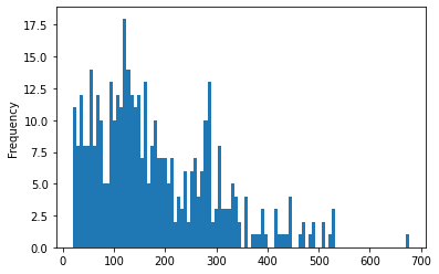
# Plot the histogram of the length column
tweets_df['length'].plot(bins=100, kind='hist') 

#Very Important 
class1 = tweets_df[tweets_df['label']==0]
#Fairly Important
class2 = tweets_df[tweets_df['label']==0]
#Slightlly important
class3 = tweets_df[tweets_df['label']==1]
#Not at all important
class4 = tweets_df[tweets_df['label']==1]

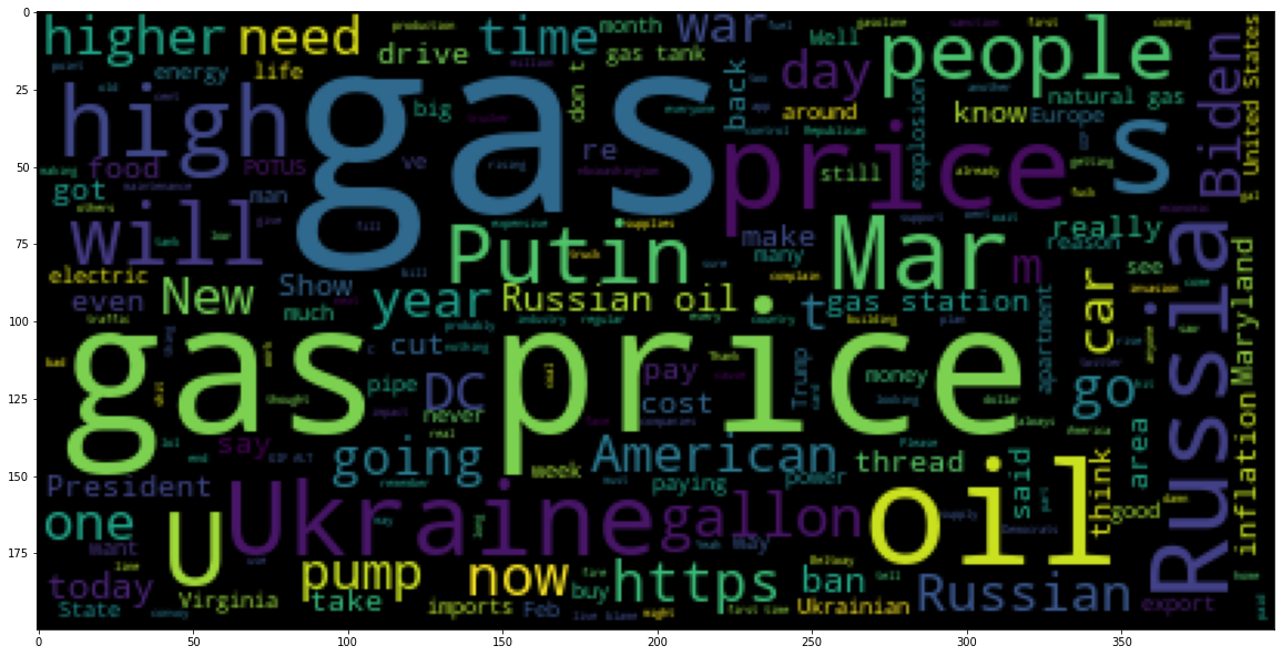
sentences = tweets_df['tweet'].tolist()
len(sentences)

420

sentences_as_one_string =" ".join(sentences)

sentences_as_one_string =sentences_as_one_string.replace('Replying', '')

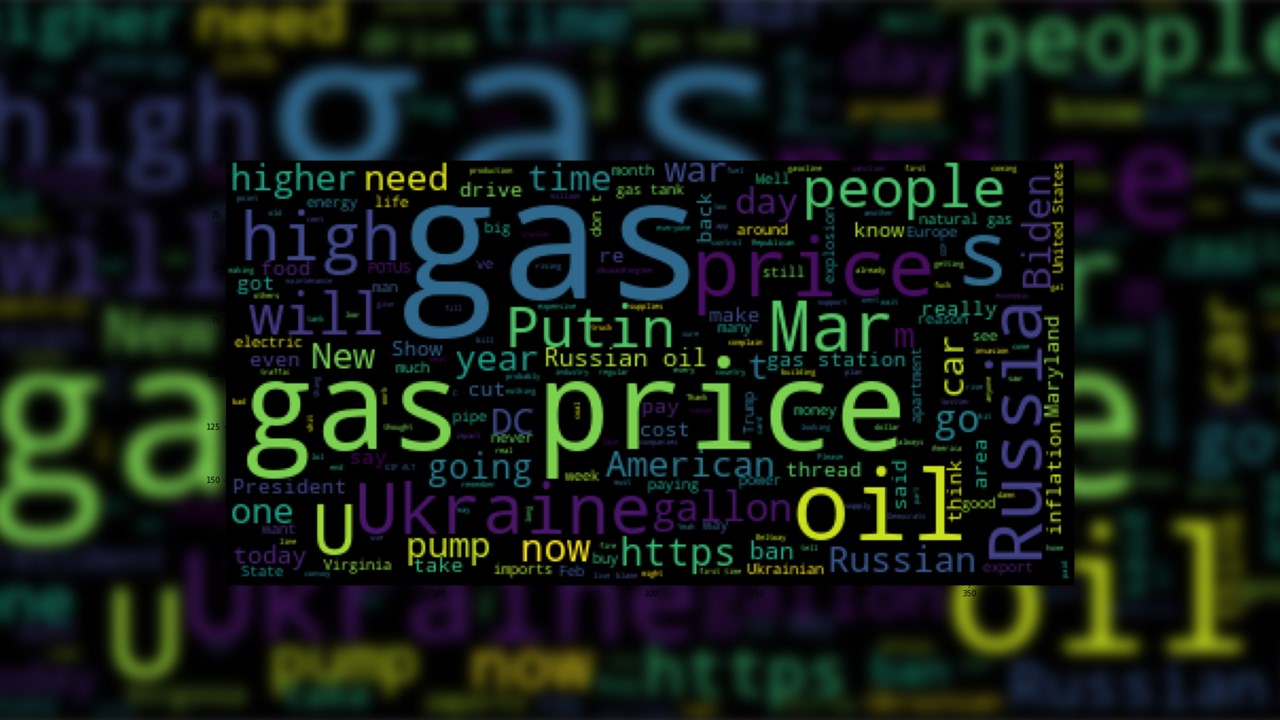
from wordcloud import WordCloud
plt.figure(figsize=(20,20))
plt.imshow(WordCloud().generate(sentences_as_one_string))

Step 7. Perform data cleaning - remove punctuation from text

Let us summarize some standard techniques to clean our text

import string
string.punctuation

'!"#$%&\'()*+,-./:;<=>?@[\\]^_`{|}~'

Test = '$I love AI & Machine learning!!'
Test_punc_removed = [char for char in Test if char not in string.punctuation]
Test_punc_removed_join = ''.join(Test_punc_removed)
Test_punc_removed_join

'I love AI  Machine learning'

Test = 'Good morning beautiful people :)... I am having fun learning Machine learning and AI!!'

Test_punc_removed = [char for char in Test if char not in string.punctuation]

# Join the characters again to form the string.
Test_punc_removed_join = ''.join(Test_punc_removed)
Test_punc_removed_join

'Good morning beautiful people  I am having fun learning Machine learning and AI'

Perform Data Cleaning - Remove Stopwords

import nltk # Natural Language tool kit 
nltk.download('stopwords')

# You have to download stopwords Package to execute this command
from nltk.corpus import stopwords
#stopwords.words('english')

[nltk_data] Downloading package stopwords to
[nltk_data]     C:\Users\rusla\AppData\Roaming\nltk_data...
[nltk_data]   Package stopwords is already up-to-date!

Test_punc_removed_join = 'I enjoy coding, programming and Artificial intelligence'
Test_punc_removed_join_clean = [word for word in Test_punc_removed_join.split() if word.lower() not in stopwords.words('english')]

Test_punc_removed_join_clean # Only important (no so common) words are left

['enjoy', 'coding,', 'programming', 'Artificial', 'intelligence']

Perform Count Vectorization (Tokenization)

from sklearn.feature_extraction.text import CountVectorizer
sample_data = ['This is the first paper.','This document is the second paper.','And this is the third one.','Is this the first paper?']
vectorizer = CountVectorizer()
X = vectorizer.fit_transform(sample_data)

print(vectorizer.get_feature_names())

['and', 'document', 'first', 'is', 'one', 'paper', 'second', 'the', 'third', 'this']

print(X.toarray())  

[[0 0 1 1 0 1 0 1 0 1]
 [0 1 0 1 0 1 1 1 0 1]
 [1 0 0 1 1 0 0 1 1 1]
 [0 0 1 1 0 1 0 1 0 1]]

Removing any URL within a string in Python

text='''
text1
text2
http://url.com/bla1/blah1/
text3
text4
http://url.com/bla2/blah2/
text5
text6
http://url.com/bla3/blah3/'
The White House Gaslights on Gas | by @njhochman  https://nationalreview.com/corner/the-white-house-gaslights-on-gas/?taid=6228b39e07024b000156be08&utm_campaign=trueanthem&utm_medium=social&utm_source=twitter…
'''

import re
text = re.sub(r'\w+:\/{2}[\d\w-]+(\.[\d\w-]+)*(?:(?:\/[^\s/]*))*', '', text)
print(text)

text1
text2

text3
text4

text5
text6

The White House Gaslights on Gas | by @njhochman  

Step 8. Create a pipeline to remove Punctuations, Stopwords and perform Count Vectorization

Let’s define a pipeline to clean up all the messages The pipeline performs the following:

1. remove urls

2. remove punctuation

3. remove stopwords

import re
def message_cleaning(message):
    message =re.sub(r'\w+:\/{2}[\d\w-]+(\.[\d\w-]+)*(?:(?:\/[^\s/]*))*', '', message)    
    Test_punc_removed = [char for char in message if char not in string.punctuation]
    Test_punc_removed_join = ''.join(Test_punc_removed)
    Test_punc_removed_join_clean = [word for word in Test_punc_removed_join.split() if word.lower() not in stopwords.words('english')]
    return Test_punc_removed_join_clean

# Let's test the newly added function
tweets_df_clean = tweets_df['tweet'].apply(message_cleaning)

print(tweets_df_clean[5]) # show the cleaned up version

['Good', 'piece', 'I’ll', 'add', 'saw', 'thread', 'yesterday', '3', 'legacy', 'media', 'reporters', 'total', 'agreement', 'there’s', 'nothing', 'get', 'gas', 'ground', 'right', 'One', 'said', 'straight', 'face', '“even', 'permit', 'issued', 'takes', 'long', 'time', 'drill”', 'National', 'Review', 'NRO', '·', 'Mar', '9', 'White', 'House', 'Gaslights', 'Gas', 'njhochman', '10', '55', '199']

print(tweets_df['tweet'][5]) # show the original version

Good piece. I’ll add that i saw a thread yesterday with 3 legacy media reporters in total agreement that there’s nothing we can do to get more gas out of the ground right now. One of them said with a straight face “even after the permit is issued, it takes a long time to drill”
National Review
@NRO
 · Mar 9
The White House Gaslights on Gas | by @njhochman  https://nationalreview.com/corner/the-white-house-gaslights-on-gas/?taid=6228b39e07024b000156be08&utm_campaign=trueanthem&utm_medium=social&utm_source=twitter…
10
55
199

from sklearn.feature_extraction.text import CountVectorizer
# Define the cleaning pipeline we defined earlier
vectorizer = CountVectorizer(analyzer = message_cleaning, dtype = np.uint8)
tweets_countvectorizer = vectorizer.fit_transform(tweets_df['tweet'])

print(vectorizer.get_feature_names())

print(tweets_countvectorizer.toarray())  

[[0 0 0 ... 0 0 0]
 [0 0 0 ... 0 0 0]
 [0 0 0 ... 0 0 0]
 ...
 [0 0 0 ... 0 0 0]
 [0 0 0 ... 0 0 0]
 [0 0 0 ... 0 0 0]]

tweets_countvectorizer.shape

(420, 3463)

X = pd.DataFrame(tweets_countvectorizer.toarray())

X.head()

	0	1	2	3	4	5	6	7	8	9	...	3453	3454	3455	3456	3457	3458	3459	3460	3461	3462
0	0	0	0	0	0	0	0	0	0	0	...	0	0	0	0	0	0	0	0	0	0
1	0	0	0	0	0	0	0	0	0	0	...	0	0	0	0	0	0	0	0	0	0
2	0	0	0	0	0	0	0	0	0	0	...	0	0	0	0	0	0	0	0	0	0
3	0	0	0	0	0	0	0	0	0	0	...	0	0	0	0	0	0	0	0	0	0
4	0	0	0	0	0	0	0	0	0	0	...	0	0	0	0	0	0	0	0	0	0

5 rows × 3463 columns

y = tweets_df['label']

Step 9. Train and evaluate a Naive Bayes Classifier Model

In statistics, naive Bayes classifiers are a family of simple “probabilistic classifiers” based on applying Bayes’ theorem with strong independence assumptions between the features. They are among the simplest Bayesian network models, but coupled with kernel density estimation, they can achieve high accuracy levels

The fundamental Naive Bayes assumption is that each feature makes an:

• independent
• equal

contribution to the outcome.

With relation to our dataset, this concept can be understood as:

• We assume that no pair of features are dependent. For example, the price being ‘Expensive’ has nothing to do with the White. Hence, the features are assumed to be independent.
• Secondly, each feature is given the same weight(or importance). For example, knowing only price and oil alone can’t predict the outcome accurately. None of the attributes is irrelevant and assumed to be contributing equally to the outcome.

X.shape

(420, 3463)

y.shape

(420,)

from sklearn.model_selection import train_test_split
X_train, X_test, y_train, y_test = train_test_split(X, y, test_size=0.2)

from sklearn.naive_bayes import MultinomialNB

NB_classifier = MultinomialNB()
NB_classifier.fit(X_train, y_train)

MultinomialNB()

from sklearn.metrics import classification_report, confusion_matrix

# Predicting the Test set results
y_predict_test = NB_classifier.predict(X_test)
fig, ax = plt.subplots(figsize=(5,5))

cm = confusion_matrix(y_test, y_predict_test)
sns.heatmap(cm, annot=True)
plt.xlabel('Predicted',fontsize=14)
plt.ylabel('True',fontsize=14)

Text(24.0, 0.5, 'True')

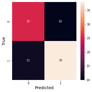
print(classification_report(y_test, y_predict_test))

              precision    recall  f1-score   support

           0       0.69      0.71      0.70        35
           1       0.79      0.78      0.78        49

    accuracy                           0.75        84
   macro avg       0.74      0.74      0.74        84
weighted avg       0.75      0.75      0.75        84

​

You can download the notebook here.

Congratulations!. You have created a dataset from twitter and analyzed which messages are relevant in according to one keyword around one geographical area.