
Logistic Regression with Python and Spark
Customer churn with Logistic Regression
A marketing agency is concerned about the number of customers stop buying their service. They need to understand who is leaving. Imagine that you are an analyst at this company and you have to find out the customers most at risk to churn an account manager.
Table of contents
The installation of Python and Pyspark and the introduction of the Logistic Regression is given here.
Logistic Regression with Python
Lets first import required libraries:
import pandas as pd
import pylab as pl
import numpy as np
import scipy.optimize as opt
from sklearn import preprocessing
%matplotlib inline
import matplotlib.pyplot as plt
Understanding the Data
churn_df = pd.read_csv("customer_churn.csv")
churn_df.head(1)
| Names | Age | Total_Purchase | Account_Manager | Years | Num_Sites | Onboard_date | Location | Company | Churn | |
|---|---|---|---|---|---|---|---|---|---|---|
| 0 | Cameron Williams | 42.0 | 11066.8 | 0 | 7.22 | 8.0 | 2013-08-30 07:00:40 | 10265 Elizabeth Mission Barkerburgh, AK 89518 | Harvey LLC | 1 |
The data is saved as customer_churn.csv. Here are the fields and their definitions:
Name : Name of the latest contact at Company
Age: Customer Age
Total_Purchase: Total Ads Purchased
Account_Manager: Binary 0=No manager, 1= Account manager assigned
Years: Totaly Years as a customer
Num_sites: Number of websites that use the service.
Onboard_date: Date that the name of the latest contact was onboarded
Location: Client HQ Address
Company: Name of Client Company
Lets select some features for the modeling. Also we change the target data type to be integer, as it is a requirement by the skitlearn algorithm:
churn_df.columns
Index(['Names', 'Age', 'Total_Purchase', 'Account_Manager', 'Years',
       'Num_Sites', 'Onboard_date', 'Location', 'Company', 'Churn'],
      dtype='object')
inputCols=['Age',
 'Total_Purchase',
 'Account_Manager',
 'Years',
 'Num_Sites','Churn']
churn_df = churn_df[inputCols]
churn_df['Churn'] = churn_df['Churn'].astype('int')
churn_df.head()
| Age | Total_Purchase | Account_Manager | Years | Num_Sites | Churn | |
|---|---|---|---|---|---|---|
| 0 | 42.0 | 11066.80 | 0 | 7.22 | 8.0 | 1 |
| 1 | 41.0 | 11916.22 | 0 | 6.50 | 11.0 | 1 |
| 2 | 38.0 | 12884.75 | 0 | 6.67 | 12.0 | 1 |
| 3 | 42.0 | 8010.76 | 0 | 6.71 | 10.0 | 1 |
| 4 | 37.0 | 9191.58 | 0 | 5.56 | 9.0 | 1 |
Lets define X, and y for our dataset:
X = np.asarray(churn_df[['Age', 'Total_Purchase', 'Account_Manager', 'Years', 'Num_Sites']])X[0:5]
array([[4.200000e+01, 1.106680e+04, 0.000000e+00, 7.220000e+00,
        8.000000e+00],
       [4.100000e+01, 1.191622e+04, 0.000000e+00, 6.500000e+00,
        1.100000e+01],
       [3.800000e+01, 1.288475e+04, 0.000000e+00, 6.670000e+00,
        1.200000e+01],
       [4.200000e+01, 8.010760e+03, 0.000000e+00, 6.710000e+00,
        1.000000e+01],
       [3.700000e+01, 9.191580e+03, 0.000000e+00, 5.560000e+00,
        9.000000e+00]])
y = np.asarray(churn_df['Churn'])y [0:5]
array([1, 1, 1, 1, 1])
Also, we normalize the dataset:
from sklearn import preprocessing
X = preprocessing.StandardScaler().fit(X).transform(X)
X[0:5]
array([[ 0.0299361 ,  0.41705373, -0.96290958,  1.52844634, -0.33323478],
       [-0.13335172,  0.76990459, -0.96290958,  0.96318219,  1.36758544],
       [-0.6232152 ,  1.172234  , -0.96290958,  1.09664734,  1.93452551],
       [ 0.0299361 , -0.85243173, -0.96290958,  1.1280509 ,  0.80064537],
       [-0.78650303, -0.36191661, -0.96290958,  0.22519844,  0.2337053 ]])
## Train/Test dataset
We split our dataset into train and test set:
from sklearn.model_selection import train_test_split
X_train, X_test, y_train, y_test = train_test_split( X, y, test_size=0.2, random_state=4)
print ('Train set:', X_train.shape,  y_train.shape)
print ('Test set:', X_test.shape,  y_test.shape)
Train set: (720, 5) (720,)Test set: (180, 5) (180,)
Lets build our model using LogisticRegression from Scikit-learn package. The version of Logistic Regression in Scikit-learn, support regularization. Regularization is a technique used to solve the overfitting problem in machine learning models.
from sklearn.linear_model import LogisticRegression
from sklearn.metrics import confusion_matrix
LR = LogisticRegression(C=0.01, solver='liblinear').fit(X_train,y_train)
LR
LogisticRegression(C=0.01, solver='liblinear')
Now we can predict using our test set:
yhat = LR.predict(X_test)
| predict_proba returns estimates for all classes, ordered by the label of classes. So, the first column is the probability of class 1, P(Y=1 | X), and second column is probability of class 0, P(Y=0 | X): |
yhat_prob = LR.predict_proba(X_test)
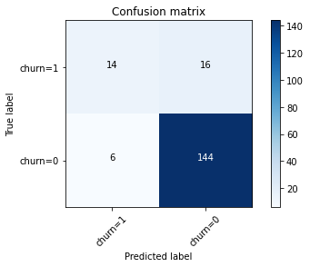
confusion matrix
Another way of looking at accuracy of classifier is to look at confusion matrix.
from sklearn.metrics import classification_report, confusion_matrix
import itertools
def plot_confusion_matrix(cm, classes,
                          normalize=False,
                          title='Confusion matrix',
                          cmap=plt.cm.Blues):
    """
    This function prints and plots the confusion matrix.
    Normalization can be applied by setting `normalize=True`.
    """
    if normalize:
        cm = cm.astype('float') / cm.sum(axis=1)[:, np.newaxis]
        print("Normalized confusion matrix")
    else:
        print('Confusion matrix, without normalization')

    print(cm)

    plt.imshow(cm, interpolation='nearest', cmap=cmap)
    plt.title(title)
    plt.colorbar()
    tick_marks = np.arange(len(classes))
    plt.xticks(tick_marks, classes, rotation=45)
    plt.yticks(tick_marks, classes)

    fmt = '.2f' if normalize else 'd'
    thresh = cm.max() / 2.
    for i, j in itertools.product(range(cm.shape[0]), range(cm.shape[1])):
        plt.text(j, i, format(cm[i, j], fmt),
                 horizontalalignment="center",
                 color="white" if cm[i, j] > thresh else "black")

    plt.tight_layout()
    plt.ylabel('True label')
    plt.xlabel('Predicted label')
print(confusion_matrix(y_test, yhat, labels=[1,0]))
[[ 14 16] [ 6 144]]
# Compute confusion matrix
cnf_matrix = confusion_matrix(y_test, yhat, labels=[1,0])
np.set_printoptions(precision=2)


# Plot non-normalized confusion matrix
plt.figure()
plot_confusion_matrix(cnf_matrix, classes=['churn=1','churn=0'],normalize= False,  title='Confusion matrix')
Confusion matrix, without normalization[[ 14 16] [ 6 144]]
print (classification_report(y_test, yhat))
precision recall f1-score support 0 0.90 0.96 0.93 150 1 0.70 0.47 0.56 30 accuracy 0.88 180 macro avg 0.80 0.71 0.74 180weighted avg 0.87 0.88 0.87 180
The average accuracy for this classifier is the average of the F1-score for both labels, which is 0.87 in our case.
Based on the count of each section, we can calculate precision and recall of each label:
-
Precision is a measure of the accuracy provided that a class label has been predicted. It is defined by: precision = TP / (TP + FP)
-
Recall is true positive rate. It is defined as: Recall = TP / (TP + FN)
we can calculate precision and recall of each class.
F1 score: Now we are in the position to calculate the F1 scores for each label based on the precision and recall of that label.
The F1 score is the harmonic average of the precision and recall, where an F1 score reaches its best value at 1 (perfect precision and recall) and worst at 0. It is a good way to show that a classifer has a good value for both recall and precision.
Logistic Regression with Pyspark
import findspark
findspark.init()
from pyspark.sql import SparkSession
spark = SparkSession.builder.appName('logregconsult').getOrCreate()
data = spark.read.csv('customer_churn.csv',inferSchema=True, header=True)
data.printSchema()
root
 |-- Names: string (nullable = true)
 |-- Age: double (nullable = true)
 |-- Total_Purchase: double (nullable = true)
 |-- Account_Manager: integer (nullable = true)
 |-- Years: double (nullable = true)
 |-- Num_Sites: double (nullable = true)
 |-- Onboard_date: string (nullable = true)
 |-- Location: string (nullable = true)
 |-- Company: string (nullable = true)
 |-- Churn: integer (nullable = true)
Check out the data
data.describe().show(1)
+-------+-----+---+--------------+---------------+-----+---------+------------+--------+-------+-----+
|summary|Names|Age|Total_Purchase|Account_Manager|Years|Num_Sites|Onboard_date|Location|Company|Churn|
+-------+-----+---+--------------+---------------+-----+---------+------------+--------+-------+-----+
|  count|  900|900|           900|            900|  900|      900|         900|     900|    900|  900|
+-------+-----+---+--------------+---------------+-----+---------+------------+--------+-------+-----+
only showing top 1 row
Format for MLlib
We’ll ues the numerical columns. We’ll include Account Manager because its easy enough, but keep in mind it probably won’t be any sort of a signal because the agency mentioned its randomly assigned!
from pyspark.ml.feature import VectorAssembler
assembler = VectorAssembler(inputCols=['Age', 'Total_Purchase', 'Account_Manager', 'Years', 'Num_Sites'],outputCol='features')
output = assembler.transform(data)
final_data = output.select('features','churn')
Test Train Split
train_churn,test_churn = final_data.randomSplit([0.7,0.3])
Fit the model
from pyspark.ml.classification import LogisticRegression
lr_churn = LogisticRegression(labelCol='churn')
fitted_churn_model = lr_churn.fit(train_churn)
training_sum = fitted_churn_model.summary
training_sum.predictions.describe().show()
+-------+-------------------+-------------------+
|summary|              churn|         prediction|
+-------+-------------------+-------------------+
|  count|                613|                613|
|   mean|0.17781402936378465|0.12887438825448613|
| stddev|  0.382668372099746|   0.33533449140226|
|    min|                0.0|                0.0|
|    max|                1.0|                1.0|
+-------+-------------------+-------------------+
Evaluate results
Let’s evaluate the results on the data set we were given (using the test data)
from pyspark.ml.evaluation import BinaryClassificationEvaluator
pred_and_labels = fitted_churn_model.evaluate(test_churn)
pred_and_labels.predictions.show()
+--------------------+-----+--------------------+--------------------+----------+| features|churn| rawPrediction| probability|prediction|+--------------------+-----+--------------------+--------------------+----------+|[22.0,11254.38,1....| 0|[4.05430795643892...|[0.98294832241403...| 0.0||[26.0,8939.61,0.0...| 0|[5.77405037803505...|[0.99690247758406...| 0.0||[28.0,8670.98,0.0...| 0|[7.23826268284963...|[0.99928195691507...| 0.0||[28.0,9090.43,1.0...| 0|[0.94821948475399...|[0.72075696108881...| 0.0||[29.0,9617.59,0.0...| 0|[3.91324626692407...|[0.98041565826455...| 0.0||[29.0,10203.18,1....| 0|[3.26598082266084...|[0.96324313418667...| 0.0||[29.0,11274.46,1....| 0|[4.17445848712145...|[0.98484954751144...| 0.0||[29.0,13255.05,1....| 0|[3.93587227636939...|[0.98084540599653...| 0.0||[30.0,8403.78,1.0...| 0|[5.44208726208492...|[0.99568823673280...| 0.0||[30.0,8677.28,1.0...| 0|[3.43610521361442...|[0.96881405579738...| 0.0||[30.0,10183.98,1....| 0|[2.48028976858033...|[0.92274845618277...| 0.0||[31.0,5304.6,0.0,...| 0|[2.67870443526006...|[0.93575828504198...| 0.0||[31.0,5387.75,0.0...| 0|[1.70594375589089...|[0.84630943026440...| 0.0||[31.0,10058.87,1....| 0|[3.92946303722257...|[0.98072461932954...| 0.0||[31.0,10182.6,1.0...| 0|[4.50159146584151...|[0.98903033715124...| 0.0||[31.0,11297.57,1....| 1|[0.60412216064385...|[0.64659882437760...| 0.0||[31.0,12264.68,1....| 0|[3.22109124776813...|[0.96162030913584...| 0.0||[32.0,5756.12,0.0...| 0|[3.45850939238844...|[0.96948389815194...| 0.0||[32.0,6367.22,1.0...| 0|[2.58844173988655...|[0.93011399503796...| 0.0||[32.0,7896.65,0.0...| 0|[2.74301964391580...|[0.93951791284489...| 0.0|+--------------------+-----+--------------------+--------------------+----------+only showing top 20 rows
Using AUC
churn_eval = BinaryClassificationEvaluator(rawPredictionCol='prediction', labelCol='churn')
auc = churn_eval.evaluate(pred_and_labels.predictions)
auc
0.7926829268292683
Predict on brand new unlabeled data
final_lr_model = lr_churn.fit(final_data)
new_customers = spark.read.csv('new_customers.csv',inferSchema=True, header=True)
new_customers.printSchema()
root
 |-- Names: string (nullable = true)
 |-- Age: double (nullable = true)
 |-- Total_Purchase: double (nullable = true)
 |-- Account_Manager: integer (nullable = true)
 |-- Years: double (nullable = true)
 |-- Num_Sites: double (nullable = true)
 |-- Onboard_date: string (nullable = true)
 |-- Location: string (nullable = true)
 |-- Company: string (nullable = true)
test_new_customers = assembler.transform(new_customers)
test_new_customers.printSchema()
root
 |-- Names: string (nullable = true)
 |-- Age: double (nullable = true)
 |-- Total_Purchase: double (nullable = true)
 |-- Account_Manager: integer (nullable = true)
 |-- Years: double (nullable = true)
 |-- Num_Sites: double (nullable = true)
 |-- Onboard_date: string (nullable = true)
 |-- Location: string (nullable = true)
 |-- Company: string (nullable = true)
 |-- features: vector (nullable = true)
final_results = final_lr_model.transform(test_new_customers)
final_results.select('Company','prediction').show()
+----------------+----------+
|         Company|prediction|
+----------------+----------+
|        King Ltd|       0.0|
|   Cannon-Benson|       1.0|
|Barron-Robertson|       1.0|
|   Sexton-Golden|       1.0|
|        Wood LLC|       0.0|
|   Parks-Robbins|       1.0|
+----------------+----------+
Now we know that we should assign Acocunt Managers to Cannon-Benson,Barron-Robertson,Sexton-GOlden, and Parks-Robbins!
You can download the notebook here
Congratulations! We have practiced Logistic Regression with Python and Spark.
Leave a comment