
Machine Learning with Python and Spark
Machine learning is the science of creating algorithms capable of learning based on the data provided to them. The primary techniques used in machine learning that we will cover here:
In the following sections, I will take a high-level look at each of these techniques.
Installation of Spark in Windows.
I will consider windows with a single computer that will simulate a cluster. In this way we test our spark codes and practice.
When we are working with Windows there is the well known bug called spark-2356, so to avoid this warning.
Go to your terminal and go to you root directory and create a directory called winutills
mkdir winutils
cd winutils
mkdir bin
cd bin
then we download winutils.exe
curl -OL https://github.com/ruslanmv/Machine-Learning-with-Python-and-Spark/raw/master/winutils.exe
then we create a empty folder
\tmp\hive
and then
c:\winutils\bin>winutils.exe chmod 777 \tmp\hive
Download Java here and during the installation choose the directory C:\jdk
C:\jdk
Download Apache Spark here . This tutorial was done by using Apache Spark 3.0.2 then
install in the following path
c:\Spark\spark-3.0.2-bin-hadoop2.7
then we go to to the main menu and Edit the system environment variables
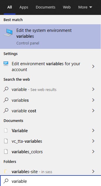
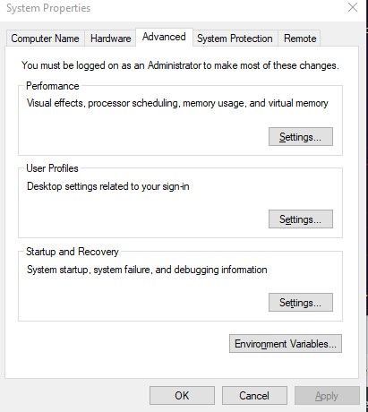
and click Environment Variables and create new variables
SPARK_HOME
C:\Spark\spark-3.0.2-bin-hadoop2.7
and
JAVA_HOME
C:\jdk-15
and
HADOOP_HOME
C:\hadoop\bin
We modify Path and we add
%SPARK_HOME%\bin
%JAVA_HOME%\bin
Cleaning the logging spark-shell
Due to we want to work without too much noise information during with spark, let us
We have to go to conf directory of spark
cd C:\Spark\spark-3.0.2-bin-hadoop2.7\conf
we copy the file
copy log4j.properties.template log4j.properties
and we edit the file log4j.properties
we change all INFO and WARN to ERROR
something like:
# Set everything to be logged to the console
log4j.rootCategory=ERROR, console
log4j.appender.console=org.apache.log4j.ConsoleAppender
log4j.appender.console.target=System.err
log4j.appender.console.layout=org.apache.log4j.PatternLayout
log4j.appender.console.layout.ConversionPattern=%d{yy/MM/dd HH:mm:ss} %p %c{1}: %m%n

# Set the default spark-shell log level to WARN. When running the spark-shell, the
# log level for this class is used to overwrite the root logger's log level, so that
# the user can have different defaults for the shell and regular Spark apps.
log4j.logger.org.apache.spark.repl.Main=ERROR

# Settings to quiet third party logs that are too verbose
log4j.logger.org.sparkproject.jetty=ERROR
log4j.logger.org.sparkproject.jetty.util.component.AbstractLifeCycle=ERROR
log4j.logger.org.apache.spark.repl.SparkIMain$exprTyper=ERROR
log4j.logger.org.apache.spark.repl.SparkILoop$SparkILoopInterpreter=ERROR
log4j.logger.org.apache.parquet=ERROR
log4j.logger.parquet=ERROR

# SPARK-9183: Settings to avoid annoying messages when looking up nonexistent UDFs in SparkSQL with Hive support
log4j.logger.org.apache.hadoop.hive.metastore.RetryingHMSHandler=FATAL
log4j.logger.org.apache.hadoop.hive.ql.exec.FunctionRegistry=ERROR
in this way we show only ERROR messages and our spark login is much clean.
Troubleshooting
To avoid problems of memory in java such as
PySpark: java.lang.OutofMemoryError: Java heap space
sudo vim $SPARK_HOME/conf/spark-defaults.conf
#uncomment the spark.driver.memory and change it according to your use. I changed it to below
spark.driver.memory 15g
# press : and then wq! to exit vim editor
If you use Spark 3.1 you should use
set PYSPARK_PYTHON=C:\Python27\bin\python.exe
Testing our setup
Let us go to the Anaconda Prompt (Anaconda3) by using cmd and we type
cd c:\Spark\spark-3.0.2-bin-hadoop2.7
we type
pyspark
we got
Welcome to
      ____              __
     / __/__  ___ _____/ /__
    _\ \/ _ \/ _ `/ __/  '_/
   /__ / .__/\_,_/_/ /_/\_\   version 3.0.2
      /_/

Using Python version 3.8.8 (default, Apr 13 2021 15:08:03)
SparkSession available as 'spark'.
>>>
type the following
>>> rdd=sc.textFile("README.md")
>>> rdd.count()
108
>>> quit
Great, you have installed Spark.
Installation of Conda
First you need to install anaconda at this link

then in the command prompt terminal we type
conda create -n pyspark python==3.7 findspark
conda activate pyspark
then in your terminal type the following commands:
conda install ipykernel
python -m ipykernel install --user --name pyspark --display-name "Python (Pyspark)"
Installing libraries
pip install -U scikit-learn
pip install numpy matplotlib pandas
then open the Jupyter notebook with the command
jupyter notebook
Then we can create a new notebook, and later we select the kernel Python (Pyspark) and then we can start.
Introduction to Machine Learning
Machine learning is the science of creating algorithms capable of learning based on the data provided to them. The primary techniques used in machine learning that we will cover here are:
In machine learning models we deal with data organized in tables that are stored in one database or in files.
The tables can be managed in Python with Dataframes. Dataframes and Datasets are the the Applications Programming Interfaces (API) that allows interact with the data.
Among the essential components of the Machine Learning models are:
-
Features: Are the columns of the tables that we will use to create our Machine Learning Model, denoted by the vector of all the feature values of the ith instance in the dataset, or in other words, the predicted value of the ith row \(\vec x^{(i)}\)
-
Prediction values: Is the variable that we want to predict, denoted by \(\hat y^{(i)} =h(\vec x^{(i)})\)
-
Number of features: Is the number of columns that we will use to create our Machine Learning Model
-
Weights: Are simple the parameters of the Machine Learning Model.
-
Hyperparameters: Are additional parameters that Machine Learning is build on.
Those are the main ingredients of the most common Machine Learning Models. In the following sections, I will take a high-level look at each of these techniques.
Linear Regression
Linear models make a prediction using a linear function of input features.
\[\hat y= w_0 + w_1 x_1 + w_2 x_2 + ... + w_n + x_n = \vec w \cdot \vec x = h_w(\vec x)\]where \(\hat y\) is the predicted value, \(n\) is the number of features, \(x_i\) is the ith feature value and \(w_j\) is the jth model parameter, where \(w_0\) is called the bias term.
To train a Linear regression model , we need to find the value \(\vec w\) that minimizes the Root Mean Square Error (RMSE)
\[RMSE(\vec x, h)=\sqrt{\frac{1}{m}\sum_{i=1}^m(h(\vec x^{(i)})-y^{(i)})^2}\]In practical linear regression problems , we can use the Mean Square Error(MSE).
The MSE of a Linear Regression hypothesis \(h_w\) on a training set \(\vec x\) is calculated by using the MSE cost function for Linear regression
\[MSE(\vec x, h_w)=\frac{1}{m}\sum_{i=1}^m(\vec w^T \vec x^{(i)})-y^{(i)})^2\]In Machine Learning, vectors are often represented as column vectors, which are 2D arrays with a single column.
If \(\vec w\) and \(\vec x\) are column vectors then the prediction is
\(\hat y = \vec w ^T \vec x\),
where \(\vec w^T\) is the transpose of \(w\) that means a row vector instead a column vector.
To find the value of \(w\) that minimizes the cost function we use the Normal Equation
\[\hat \theta = (\vec x^T \vec x)^{-1} \vec x^T \vec y\]where \(\hat \theta\) is the value of \(\vec w\) that minimizes the cost function, and \(\vec y\) is the vector of target values.
There are different techniques that allows us minimizes the cost function. Among them the most used is the Gradient descent
We need to calculate how much the cost function will change if you change \(w_j\) a little bit. This is possible with the partial derivative
\[\frac{\partial }{\partial w_j}MSE(\vec w)=\frac{2}{m}\sum_{i=1}^m(\vec w^T \vec x^{(i)})-y^{(i)})x_j^{(i)}\]Instead use the partials individually we can compute the gradient vector
\[\nabla_W MSE(W)=\frac{2}{m}X^T(XW-y)\]then we can use the gradient step
\[W^{(step+1)}=W-\eta \nabla_W MSE(W)\]where eta \(\eta\) is the hyperparameter called learning rate.
Now that we have seen at high level the idea of linear regression, we will discuss a problem or linear regression by using Spark and Python
We will examine a dataset with Ecommerce Customer Data for a company’s website. Then we will build a regression model that will predict the customer’s yearly spend on the company’s product, to see more you continue here
Logistic Regression
Linear Regression is suited for estimating continuous values (e.g. estimating house price), it is not the best tool for predicting the class of an observed data point. In order to estimate the class of a data point, we need some sort of guidance on what would be the most probable class for that data point. For this, we use Logistic Regression.
As you know, Linear regression finds a function that relates a continuous dependent variable, y, to some predictors (independent variables \(x_1, x_2\), etc.). For example, Simple linear regression assumes a function of the form:
\[y = w_0 + w_1 x_1 + w_2 x_2 + \cdots\]and finds the values of parameters \(w_0, ws_1, w_2\), etc, where the term \(w_0\) is the “intercept”. It can be generally shown as:
\[h_w(𝑥) = w^TX\]Logistic Regression is a variation of Linear Regression, useful when the observed dependent variable, y, is categorical. It produces a formula that predicts the probability of the class label as a function of the independent variables.
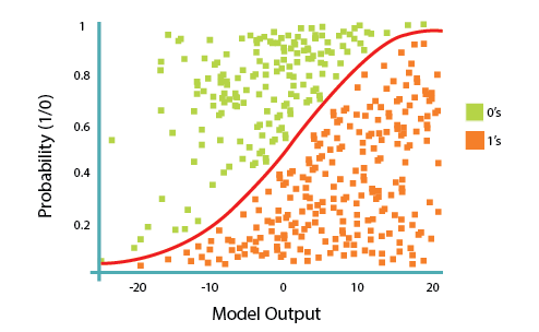
Logistic regression fits a special s-shaped curve by taking the linear regression and transforming the numeric estimate into a probability with the following function, which is called sigmoid function 𝜎:
\[h_\vec w(\vec x) = \sigma({\vec w^T \vec X}) = \frac {e^{(w_0 + w_1 x_1 + w_2 x_2 +...)}}{1 + e^{(w_0 + w_1 x_1 + w_2 x_2 +\cdots)}}\]or probability of a class 1:
\[P(Y=1|X) = \sigma({w^TX}) = \frac{e^{w^TX}}{1+e^{w^TX}}\]Where the logistic is a a sigmoid function that outputs a number between 0 and 1
\[\sigma(t)=\frac{1}{1+exp(-t)}\]So, briefly, Logistic Regression passes the input through the logistic/sigmoid but then treats the result as a probability:
The objective of Logistic Regression algorithm, is to find the best parameters W, for
\[ℎ_W(x) = \sigma({W^TX})\]in such a way that the model best predicts the class of each case.
Now that we have seen at high level the idea of logistic regression, we will discuss a problem by using Spark and Python here
Decision Trees
Decision Trees are Machine Learning Algorithms that perform both classification and regression tasks.
Essentially , they learn a hierarchy of if/else questions leading to a decision.
A decision tree takes as input an object or situation described by a set of attributes and returns a decision, the predicted output value for the input.
The input attributes can be discrete or continuous. For now, we assume discrete inputs.
The output value can also be discrete or continuous; learning a discrete-valued function is called classification learning; learning a continuous function is called regression. We will concentrate on Boolean classificaction, wherein each example is classified as true (positive) or false (negative).
A decision tree reaches its decision by performing a sequence of tests. Each internal node in the tree corresponds to a test of the value of one of the properties, and the branches from the node are labeled with the possible values of the test.
Each leaf node in the tree specifies the value to be returned if that leaf is reached.
The scheme used in decision tree learning for selecting attributes is designed to minimize the depth of the final tree.
The idea is to pick the attribute that goes as far as possible toward providing an exact classification of the examples.
A perfect attribute divides the examples into sets that are all positive or all negative. The Patrons attribute is not perfect, but it is fairly good.
A really useless attribute, such as Type, leaves the example sets with roughly the same proportion of positive and negative examples as the original set.
Now that we have seen the idea of Decision Trees, let us see an example to understand better this technique by using Spark and Python here
Clustering
There are many models for clustering out there. We will be presenting the model that is considered one of the simplest models amongst them. Despite its simplicity, the K-means is vastly used for clustering in many data science applications, especially useful if you need to quickly discover insights from unlabeled data.
Some real-world applications of k-means:
- Customer segmentation
- Understand what the visitors of a website are trying to accomplish
- Pattern recognition
- Machine learning
- Data compression
K-means is an unsupervised learning algorithm used for clustering problem whereas KNN is a supervised learning algorithm used for classification and regression problem. This is the basic difference between K-means and KNN algorithm. … It makes predictions by learning from the past available data.
In this sense, it is important to consider the value of k. But hopefully from this diagram, you should get a sense of what the K-Nearest Neighbors algorithm is. It considers the ‘K’ Nearest Neighbors (points) when it predicts the classification of the test point.
Now that we have seen the idea of clustering, let us discuss a problem by using Spark and Python here
Collaborative Filtering
Recommendation systems are a collection of algorithms used to recommend items to users based on information taken from the user. These systems have become ubiquitous can be commonly seen in online stores, movies databases and job finders. We will explore recommendation systems based on Collaborative Filtering and implement simple version of one using Python and the Pandas library.
With Collaborative filtering we make predictions (filtering) about the interests of a user by collecting preferences or taste information from many users (collaborating). The underlying assumption is that if a user A has the same opinion as a user B on an issue, A is more likely to have B’s opinion on a different issue x than to have the opinion on x of a user chosen randomly.
The image below (from Wikipedia) shows an example of collaborative filtering. At first, people rate different items (like videos, images, games). Then, the system makes predictions about a user’s rating for an item not rated yet. The new predictions are built upon the existing ratings of other users with similar ratings with the active user.

Spark MLlib library for Machine Learning provides a Collaborative Filtering implementation by using Alternating Least Squares. .
The first technique we’re going to take a look at is called Collaborative Filtering, which is also known as User-User Filtering.
As hinted by its alternate name, this technique uses other users to recommend items to the input user.
It attempts to find users that have similar preferences and opinions as the input and then recommends items that they have liked to the input. There are several methods of finding similar users (Even some making use of Machine Learning), and the one we will be using here is going to be based on the Pearson Correlation Function.
Now that we have seen the idea of recommendations, let us discuss a problem by using Spark and Python here
Congratulations! We have an idea about some models in Machine Learning.
Leave a comment