
Essential PySpark Tutorial to Get You Started in Big Data
Today we are going to practice some exercises and questions in Pyspark by using a ready Jupyter Notebook Instance in a Docker Container I have collected some relevant questions and answers to understand better how it works Pyspark. In order to answer the exercises we are going to use a docker container with Pyspark. Let us install Docker in your computer Step 1. Install Docker desktop in you computer.
https://www.docker.com/products/docker-desktop
after installed we restart our computer and then we open docker desktop and then open a terminal
Step 2. Run the following command
docker run -p 8888:8888 --user root -e GRANT_SUDO=yes ruslanmv/pyspark-notebook:3.1.2
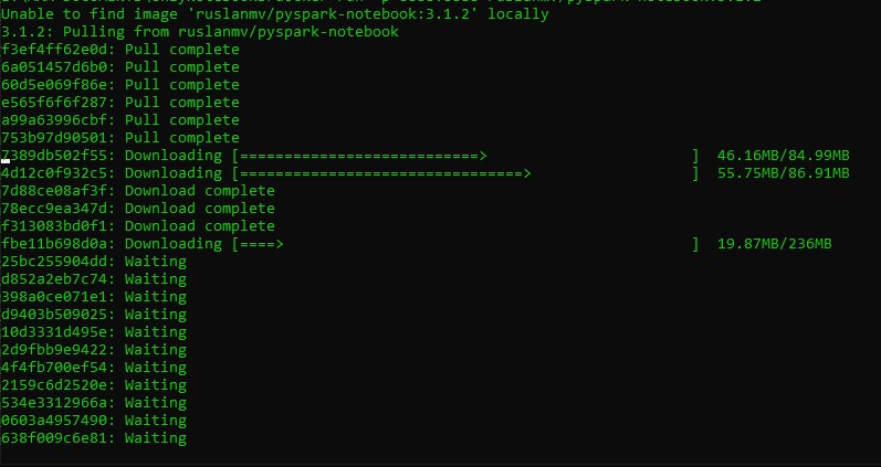
after is done you will get adirection something like
http://127.0.0.1:8888/?token=d81f55db1541bb5ed56d91227ae88997e65bee6934fd5bbb
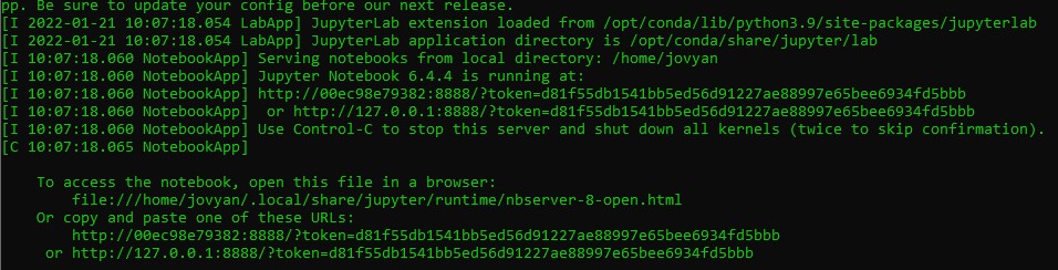
copy your address a, open your favorite web browser and paste and press enter. Then click open new Terminal
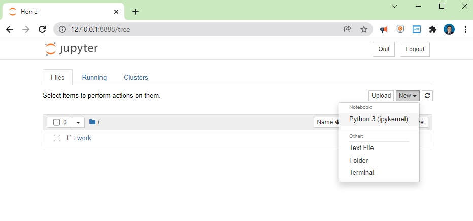
and type
git clone https://github.com/ruslanmv/Tutorial-of-Pyspark-with-Jupyter-Notebook.git
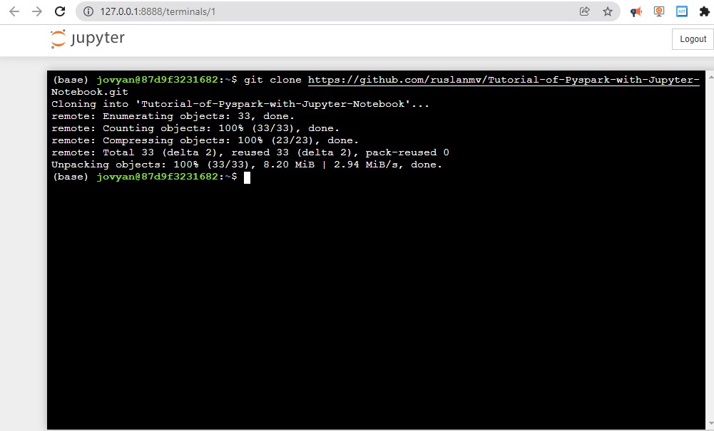
Then return to your home tree and open the created folder Tutorial-of-Pyspark-with-Jupyter-Notebook and open the Tutorial-Pyspark-Final.ipynb file
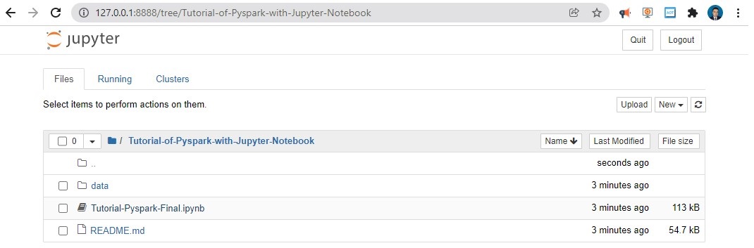
and follow the notebook by pressing shift+enter on each cell. Great, now we are ready to answer some questions!
What is PySpark?
PySpark is an Apache Spark interface in Python. It is used for collaborating with Spark using APIs written in Python.
It also supports Spark’s features like Spark DataFrame, Spark SQL, Spark Streaming, Spark MLlib and Spark Core.
What is Findspark used for?
Findspark can add a startup file to the current IPython profile so that the environment vaiables will be properly set and pyspark will be imported upon IPython startup. This file is created when edit_profile is set to true. Findspark can also add to th
import findspark
findspark.init()
How to Initializing Spark?
The first thing a Spark program is to create a SparkContext object, which tells Spark how to access a cluster.
When we run any spark application, the driver program starts, which has the main() function and the SparkContext gets initiated here
from pyspark.sql import SparkSession
spark = SparkSession \
    .builder \
    .appName("Python Spark SQL basic example") \
    .config("spark.some.config.option", "some-value") \
    .getOrCreate()
Sparksession is the Spark Entry Point
It contains the former
- Sparkcontext
- SparkConf
- Sqlcontext
- Hivecontext
- Streaming Context
Used for:
- metadata acess
- read data
- conf session
- manage cluster resources (YARN,MESOS)
Determine Spark version
# spark
print(f"Spark version = {spark.version}")
Spark version = 3.0.2
What is PySpark SparkContext?
PySpark SparkContext is an initial entry point of the spark functionality. It also represents Spark Cluster Connection and can be used for creating the Spark RDDs (Resilient Distributed Datasets) and broadcasting the variables on the cluster.
from pyspark import SparkContext
sc = SparkContext.getOrCreate()
sc.version #Retrieve SparkContext version
'3.0.2'
sc.pythonVer #Retrieve Python version
'3.8'
sc.master #Master URL to connect to
'local[*]'
str(sc.sparkHome) #Path where Spark is installed an worker nodes
'None'
str(sc.sparkUser()) #Retrieve name of the Spark User running SparkContext
'rusla'
sc.appName #Return application name
'Python Spark SQL basic example'
sc.applicationId #Retrieve application ID
'local-1643013259822'
sc.defaultParallelism #Return default level of parallelism
12
sc.defaultMinPartitions #Default minimum number of partitions for RDDs
2
sc.getConf()
<pyspark.conf.SparkConf at 0x19d93300910>
#Apache Spark allow have one Sparkcontect on one node
sc.stop()
Configuration
from pyspark import SparkConf, SparkContext
conf = (SparkConf()
            .setMaster("local")
            .setAppName("My app")
            .set("spark.executor.memory","1g" ) )
sc = SparkContext(conf = conf)
Using The Shell
In the PySpark shell, a special interpreter aware SparkContext is already created in the variable called sc.
$ ./bin/spark shell --master local[2]
$ ./bin/pyspark --master local[4] --py files code.py
Set which master the context connects to with the –master argument, and add Python .zip, .egg or .py files to the runtime path by passing a comma separated list to –py-files
What is spark-submit? Spark-submit is a utility to run a pyspark application job by specifying options and configurations.
where configurations are:
spark-submit \
--master <master-url> \
--deploy-mode <deploy-mode> \
--conf <key<=<value> \
--driver-memory <value>g \
--executor-memory <value>g \
--executor-cores <number of cores> \
--jars <comma separated dependencies> \
--packages <package name> \
--py-files \
<application> <application args>
How you can run pyspark program?
You can use jupyter notebook as in this tutorial we are doing, or just create a python file under bin folder. Write above codes in the .py file. Execute the file using
spark-submit example.py
What are the Data structures in Pyspark?
- RDD : Data is organized into named columns, like a table in a relational database. (untyped)
- Transformations
- collect : RDD–> LIST
- MAP : RDD –> PipelinedRDD
- filter : RDD –> LIST
- Actions
- Transformations
-
DF : DataFrame is an immutable distributed collection of data (untyped)
- DS : Dataset (typed)
DataFrame and Dataset APIs are built on top of the Spark SQL engine, it uses Catalyst to generate an optimized logical and physical query plan.
Across R, Java, Scala, or Python DataFrame/Dataset APIs, all relation type queries undergo the same code optimizer, providing the space and speed efficiency.
Whereas the Dataset[T] typed API is optimized for data engineering tasks, the untyped Dataset[Row] (an alias of DataFrame) is even faster and suitable for interactive analysis.
How to read a .csv file and infer schema?
from pyspark.sql import SparkSession
# Create a SparkSession
spark = (SparkSession
  .builder
  .appName("App")
  .getOrCreate())
# Path to data set
csv_file = "data/departuredelays.csv"
df = (spark.read.format("csv")
  .option("inferSchema", "true")
  .option("header", "true")
  .load(csv_file))
df.createOrReplaceTempView("us_delay_flights_tbl")
Now that we have a temporary view, we can issue SQL queries using Spark SQL. These queries are no different from those you might issue against a SQL table in, say, a MySQL or PostgreSQL database.
Next, we’ll find all flights between San Francisco (SFO) and Chicago (ORD) with at least a two-hour delay:
spark.sql("""SELECT date, delay, origin, destination
FROM us_delay_flights_tbl
WHERE delay > 120 AND ORIGIN = 'SFO' AND DESTINATION = 'ORD'
ORDER by delay DESC""").show(10)
+-------+-----+------+-----------+
|   date|delay|origin|destination|
+-------+-----+------+-----------+
|2190925| 1638|   SFO|        ORD|
|1031755|  396|   SFO|        ORD|
|1022330|  326|   SFO|        ORD|
|1051205|  320|   SFO|        ORD|
|1190925|  297|   SFO|        ORD|
|2171115|  296|   SFO|        ORD|
|1071040|  279|   SFO|        ORD|
|1051550|  274|   SFO|        ORD|
|3120730|  266|   SFO|        ORD|
|1261104|  258|   SFO|        ORD|
+-------+-----+------+-----------+
only showing top 10 rows
As with the DataFrame and Dataset APIs, with the spark.sql interface you can conduct common data analysis operations
We’ll find all flights whose distance is greater than 1,000 miles:
from pyspark.sql.functions import col, desc
(df.select("distance", "origin", "destination")
  .where(col("distance") > 1000)
  .orderBy(desc("distance"))).show(10)
+--------+------+-----------+
|distance|origin|destination|
+--------+------+-----------+
|    4330|   HNL|        JFK|
|    4330|   HNL|        JFK|
|    4330|   HNL|        JFK|
|    4330|   HNL|        JFK|
|    4330|   HNL|        JFK|
|    4330|   HNL|        JFK|
|    4330|   HNL|        JFK|
|    4330|   HNL|        JFK|
|    4330|   HNL|        JFK|
|    4330|   HNL|        JFK|
+--------+------+-----------+
only showing top 10 rows
What are RDDs in PySpark?
RDDs expand to Resilient Distributed Datasets. These are the elements that are used for running and operating on multiple nodes to perform parallel processing on a cluster. Since RDDs are suited for parallel processing, they are immutable elements. This means that once we create RDD, we cannot modify it. RDDs are also fault-tolerant which means that whenever failure happens, they can be recovered automatically. Multiple operations can be performed on RDDs to perform a certain task.
- RDD is a distributed collection of data elements without any schema
- No in-built optimization engine for RDDs
- We need to define the schema manually.
- RDD is slower than both Dataframes and Datasets to perform simple operations like grouping the data
Loading Data
Parallelized Collection
rdd = sc.parallelize([('a',7),('a',2),('b',2)])
rdd2 = sc.parallelize([('a',2),('d',1),('b',1)])
rdd3 = sc.parallelize(range(100))
rdd4 = sc.parallelize([("a",["x","y","z"]),
                            ("b",["p","r"])])
External Data
Read either one text file from HDFS.a local file system or or any Hadoop-supported file system URI with textFile(). or read in a directory of text files with wholeTextFiles()
textFile = sc.textFile("data/people.txt")
textFile2 = sc.wholeTextFiles( "data/Orders")
Retrieving RDD Information
Basic Information
rdd.getNumPartitions() #List the number of partitions
1
rdd.count() #Count ROD instances 3
3
rdd.countByKey() #Count ROD instances by key
defaultdict(int, {'a': 2, 'b': 1})
rdd.countByValue() #Count ROD instances by value
defaultdict(int, {('a', 7): 1, ('a', 2): 1, ('b', 2): 1})
rdd.collectAsMap() #Return (key,value) pairs as a dictionary
{'a': 2, 'b': 2}
rdd3.sum() #Sum of ROD elements 4950
4950
sc.parallelize([]).isEmpty() #Check whether ROD is empty
True
Summary
rdd3.max() #Maximum value of ROD elements 99
99
rdd3.min() #Minimum value of ROD elements
0
rdd3.mean() #Mean value of ROD elements
49.5
rdd3.stdev() #Standard deviation of ROD elements
28.86607004772212
rdd3.variance() #Compute variance of ROD elements 833.25
833.25
rdd3.histogram(3) #Compute histogram by bins
([0, 33, 66, 99], [33, 33, 34])
rdd3.stats() #Summary statistics (count, mean, stdev, max & min)
(count: 100, mean: 49.5, stdev: 28.86607004772212, max: 99.0, min: 0.0)
Applying Functions
#Apply a function to each ROD element
rdd.map(lambda x: x+(x[1],x[0])).collect()
[('a', 7, 7, 'a'), ('a', 2, 2, 'a'), ('b', 2, 2, 'b')]
#Apply a function to each ROD element and flatten the result
rdd5 = rdd.flatMap(lambda x: x+(x[1],x[0]))
rdd5.collect()
['a', 7, 7, 'a', 'a', 2, 2, 'a', 'b', 2, 2, 'b']
Selecting Data
rdd.collect() #Return a list with all ROD elements
[('a', 7), ('a', 2), ('b', 2)]
rdd.take(2) #Take first 2 ROD elements
[('a', 7), ('a', 2)]
rdd.first() #Toke first ROD element
('a', 7)
rdd.top(2) #Take top 2 ROD elements
[('b', 2), ('a', 7)]
Creation of RDD using textFile API
from pyspark.sql import SparkSession
spark = SparkSession \
    .builder \
    .appName("Python Spark SQL basic example") \
    .config("spark.some.config.option", "some-value") \
    .getOrCreate()
#  We can create a RDD from file
rdd6 = spark.sparkContext.textFile('data/people.txt')
#Now that it is created the rdd we can take the first 5 elements with take()
rdd6.take(5)
['Michael, 29', 'Andy, 30', 'Justin, 19']
#We can print the elements that we have taken
for i in rdd6.take(5):
    print(i)
Michael, 29
Andy, 30
Justin, 19
Get the Number of Partitions in the RDD
rdd6.getNumPartitions()
1
Create a RDD from a Python List
lst = [1,2,3,4,5,6,7]
rdd7 = spark.sparkContext.parallelize(lst)
for i in rdd7.take(5) :
    print(i)
1
2
3
4
5
Creation of rdd manually
rdd8 = sc.parallelize(
    [('Amber', 22), ('Alfred', 23), ('Skye',4), ('Albert', 12),
     ('Amber', 9)])
print(type(rdd8))
rdd8.collect()
<class 'pyspark.rdd.RDD'>


[('Amber', 22), ('Alfred', 23), ('Skye', 4), ('Albert', 12), ('Amber', 9)]
Create a RDD from local file
lst = open('data/people.txt').read().splitlines()
lst[0:10]
rdd9 = spark.sparkContext.parallelize(lst)
for i in rdd9.take(5) : print(i)
Michael, 29
Andy, 30
Justin, 19
#reading from file taking 4 partitions
data_from_file = sc.textFile('data/people.txt',4)
type(data_from_file)
pyspark.rdd.RDD
how many partitions
data_from_file.getNumPartitions()
4
Create RDD using textFile API and a defined number of partitions
rdd10 = spark.sparkContext.textFile('data/Orders',10)
for i in rdd10.take(5) : print(i)
1,2013-07-25 00:00:00.0,11599,CLOSED
2,2013-07-25 00:00:00.0,256,PENDING_PAYMENT
3,2013-07-25 00:00:00.0,12111,COMPLETE
4,2013-07-25 00:00:00.0,8827,CLOSED
5,2013-07-25 00:00:00.0,11318,COMPLETE
Create RDD from range function
lst1 = range(10)
rdd11 = spark.sparkContext.parallelize(lst1)
for i in rdd11.take(5) : print(i)
0
1
2
3
4
What are Dataframes?
It was introduced first in Spark version 1.3 to overcome the limitations of the Spark RDD. Spark Dataframes are the distributed collection of the data points, but here, the data is organized into the named columns
- It is also the distributed collection organized into the named columns
- It uses a catalyst optimizer for optimization.
- It will automatically find out the schema of the dataset.
- It performs aggregation faster than both RDDs and Datasets.
Create RDD from a DataFrame
df=spark.createDataFrame(data=(('robert',35),('Mike',45)),schema=('name','age'))
df.printSchema()
df.show()
rdd11= df.rdd
type(rdd11)
for i in rdd11.take(2) : print(i)
root
 |-- name: string (nullable = true)
 |-- age: long (nullable = true)

+------+---+
|  name|age|
+------+---+
|robert| 35|
|  Mike| 45|
+------+---+

Row(name='robert', age=35)
Row(name='Mike', age=45)
What are Datasets?
Spark Datasets is an extension of Dataframes API with the benefits of both RDDs and the Datasets. It is fast as well as provides a type-safe interface.
- It is an extension of Dataframes with more features like type-safety and object-oriented interface.
- It uses a catalyst optimizer for optimization.
- It will automatically find out the schema of the dataset.
- Dataset is faster than RDDs but a bit slower than Dataframes.
What type of operation has Pyspark?
The operations can be of 2 types, actions and transformation.
What is Transformation in Pyspark?
Transformation: These operations when applied on RDDs result in the creation of a new RDD. Some of the examples of transformation operations are filter, groupBy, map.
![]()
Filtering
rdd.filter(lambda x: "a" in x).collect() #Filter the ROD
[('a', 7), ('a', 2)]
rdd5.distinct().collect() #Return distinct ROD values
['a', 7, 2, 'b']
rdd.keys().collect() #Return (key,value) RDD's keys
['a', 'a', 'b']
def g(x): print(x)
rdd.foreach(g) #Apply a function to all ROD elements
Reshaping Data
Reducing
rdd.reduceByKey(lambda x,y : x+y).collect() #Merge the rdd values for each key
[('a', 9), ('b', 2)]
rdd.reduce(lambda a, b: a+b) #Merge the rdd values
('a', 7, 'a', 2, 'b', 2)
Grouping by
groupped=rdd3.groupBy(lambda x: x % 2) \
 .mapValues(list)\
 .collect()
rdd.groupByKey() \
 .mapValues(list)\
 .collect()
[('a', [7, 2]), ('b', [2])]
Aggregating
seqOp = (lambda x,y: (x[0]+y,x[1]+1))
combOp = (lambda x,y:(x[0]+y[0],x[1]+y[1]))
#Aggregate RDD elements of each partition and then the results
rdd3.aggregate((0,0),seqOp,combOp)
(4950, 100)
#Aggregate values of each RDD key
rdd.aggregateByKey((0,0),seqOp,combOp).collect()
[('a', (9, 2)), ('b', (2, 1))]
#Create tuples of RDD elements by applying a function
tuple=rdd3.keyBy(lambda x: x+x).collect()
Mathematical Operations
rdd.subtract(rdd2).collect() #Return each rdd value not contained in rdd2
[('a', 7), ('b', 2)]
#Return each (key,value) pair of rdd2 with no matching key in rdd
rdd2.subtractByKey(rdd).collect()
[('d', 1)]
rdd.cartesian(rdd2).collect() #Return the Cartesian product of rdd and rdd2
[(('a', 7), ('a', 2)),
 (('a', 7), ('d', 1)),
 (('a', 7), ('b', 1)),
 (('a', 2), ('a', 2)),
 (('a', 2), ('d', 1)),
 (('a', 2), ('b', 1)),
 (('b', 2), ('a', 2)),
 (('b', 2), ('d', 1)),
 (('b', 2), ('b', 1))]
Sort
rdd2.sortBy(lambda x: x[1]).collect() #Sort ROD by given function
[('d', 1), ('b', 1), ('a', 2)]
rdd2.sortByKey().collect() #Sort (key, value) ROD by key
[('a', 2), ('b', 1), ('d', 1)]
Let us take an example to demonstrate transformation operation by considering filter() operation:
words_list = sc.parallelize (
  ["pyspark",
  "interview",
  "questions"]
)
filtered_words = words_list.filter(lambda x: 'interview' in x)
filtered = filtered_words.collect()
print(filtered)
['interview']
What is map?
Perform row level transformations where one record transforms into another record. Number of records in input is equal to output, Return a new RDD by applying a function to each element of this RDD
View RDD contents in Python Spark take / collect
When you call collect() or take(), you get back a list of elements in the rdd. You can then print these values as you would any normal python list.
rdd.take(3)
[('a', 7), ('a', 2), ('b', 2)]
a=data_from_file.collect()
type(a)
list
a=data_from_file.map(lambda row: row)
b=a.collect()
print(type(b))
print(b)
<class 'list'>
['Michael, 29', 'Andy, 30', 'Justin, 19']
Project all the Order_ids by using map
ord = sc.textFile('data/Orders')
ordMap = ord.map(lambda x : x.split(',')[0])
for i in ordMap.take(5) : print(i)
1
2
3
4
5
Project all the Orders and their status
ord.map(lambda x : (x.split(',')[0],x.split(',')[3])).take(5)
[('1', 'CLOSED'),
 ('2', 'PENDING_PAYMENT'),
 ('3', 'COMPLETE'),
 ('4', 'CLOSED'),
 ('5', 'COMPLETE')]
Combine Order id and status with ‘#’
ord.map(lambda x : x.split(',')[0] + '#' + x.split(',')[3]).take(5)
['1#CLOSED', '2#PENDING_PAYMENT', '3#COMPLETE', '4#CLOSED', '5#COMPLETE']
Convert the Order date into YYYY/MM/DD Format.
ord.map(lambda x : x.split(',')[1].split(' ')[0].replace('-','/')).first()
'2013/07/25'
Print Five elements of the RDD
map = ord.map(lambda x: (x, 1))
mapreduce = map.reduceByKey(lambda x,y: x+y)
result = mapreduce.collect()
top5 = result[:5]
top5
[('1,2013-07-25 00:00:00.0,11599,CLOSED', 1),
 ('2,2013-07-25 00:00:00.0,256,PENDING_PAYMENT', 1),
 ('3,2013-07-25 00:00:00.0,12111,COMPLETE', 1),
 ('4,2013-07-25 00:00:00.0,8827,CLOSED', 1),
 ('5,2013-07-25 00:00:00.0,11318,COMPLETE', 1)]
Applied user defined function to convert status into lowercase.
def lowerCase(str):
    return str.lower()
ord.map(lambda x : lowerCase(x.split(',')[3])).first()
'closed'
What is flatMap?
Return a new RDD by first applying a function to all elements of this RDD, and then flattening the results Similar to map, but each input item can be mapped to 0 or more output items (so func should return a Seq rather than a single item). Number of records in input is less than or equal to output.
Word count in orders file using flatMap
ord = sc.textFile('data/Orders')
wordCount = ord.flatMap(lambda x : x.split(',')).map(lambda w : (w,1)).reduceByKey(lambda x,y : x+y)
#### flatMap [used to extract word]
a=data_from_file.flatMap(lambda row: row)
b=a.collect()
print(type(b))
print(b)
#a.collect()
<class 'list'>
['M', 'i', 'c', 'h', 'a', 'e', 'l', ',', ' ', '2', '9', 'A', 'n', 'd', 'y', ',', ' ', '3', '0', 'J', 'u', 's', 't', 'i', 'n', ',', ' ', '1', '9']
#FLATMAP
wordCount =data_from_file.flatMap(lambda line: line.split()).map(lambda word: (word,1)).reduceByKey(lambda a,b: a+b)
print('wordCount: %s ' % wordCount.collect())
wordCount: [('Andy,', 1), ('Michael,', 1), ('30', 1), ('29', 1), ('Justin,', 1), ('19', 1)]
What is filter?
Return a new dataset formed by selecting those elements of the source on which func returns true.
Print all the orders which are closed or Complete and ordered in the year 2013 by using filter
ord = sc.textFile('Orders')
filteredOrd = ord.filter(lambda x : (x.split(',')(3) in ("CLOSED","COMPLETE")) and (x.split(',')(1).split('-')(0) == '2014'))
# filtering
data_from_file.filter(lambda row: row[0] == 'A').collect()
['Andy, 30']
# distinct()
data_from_file.map(lambda row: row[0]).distinct().collect()
['J', 'M', 'A']
What is mapValues?
The difference with map is map operates on the entire record.
rdd = sc.parallelize((("a", (1,2,3)), ("b", (3,4,5)),("a", (1,2,3,4,5))))
def f(x): return len(x)
rdd.mapValues(f).collect()
[('a', 3), ('b', 3), ('a', 5)]
What is join in pyspark?
When called on datasets of type (K, V) and (K, W), returns a dataset of (K, (V, W)) pairs with all pairs of elements for each key.
Find the subtotal for each ORDER_CUSTOMER_ID by using join
ord = sc.textFile('data/Orders')
ordItems = sc.textFile('data/Order_items')
ordMap=ord.map(lambda x : (x.split(',')(0),x.split(',')(2)))
ordItemsMap=ordItems.map(lambda x : (x.split(',')(1),x.split(',')(4)))
findSubtotalForCust = ordMap.join(ordItemsMap)
join / leftouterjoin / intersection
rdd1 = sc.parallelize([('a', 1), ('b', 4), ('c',10)])
rdd2 = sc.parallelize([('a', 4), ('a', 1), ('b', '6'), ('d', 15)])

rdd3 = rdd1.leftOuterJoin(rdd2)
rdd3.take(5)
[('b', (4, '6')), ('c', (10, None)), ('a', (1, 4)), ('a', (1, 1))]
rdd4 = rdd1.join(rdd2)
rdd4.collect()
[('b', (4, '6')), ('a', (1, 4)), ('a', (1, 1))]
reduce
data_from_file.map(lambda row: row[2]).reduce(lambda x, y: x + y)
'cds'
data_from_file.count()
3
What is cogroup in pyspark?
When called on datasets of type (K, V) and (K, W), returns a dataset of (K, (Iterable, Iterable)) tuples.
Give me an example of cogroup
x = sc.parallelize((("a", 1), ("b", 4)))
y = sc.parallelize((("a", 2)))
xy = x.cogroup(y)
What is cartesian in Pyspark?
Perform a cross join. Give me an example of cartesion in Pyspark
rdd13 = sc.parallelize((1,3,2))
sorted(rdd.cartesian(rdd).collect())
[(('a', (1, 2, 3)), ('a', (1, 2, 3))),
 (('a', (1, 2, 3)), ('a', (1, 2, 3, 4, 5))),
 (('a', (1, 2, 3)), ('b', (3, 4, 5))),
 (('a', (1, 2, 3, 4, 5)), ('a', (1, 2, 3))),
 (('a', (1, 2, 3, 4, 5)), ('a', (1, 2, 3, 4, 5))),
 (('a', (1, 2, 3, 4, 5)), ('b', (3, 4, 5))),
 (('b', (3, 4, 5)), ('a', (1, 2, 3))),
 (('b', (3, 4, 5)), ('a', (1, 2, 3, 4, 5))),
 (('b', (3, 4, 5)), ('b', (3, 4, 5)))]
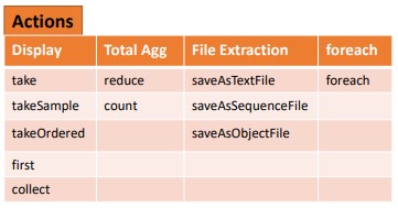
Give me some Aggregation Operations in Spark
There are several APIs to perform aggregation Operations. •
-
Total aggregations – reduce, count (Actions) •
-
By Key aggregations – reduceByKey, aggregrateByKey, groupByKey, countByKey (Transformations)
What is the aggregation reduce?
Reduces the elements of this RDD using the specified commutative and associative binary operator. Currently reduces partitions locally
What is the aggregration count?
Return the number of elements in this RDD.
from pyspark.sql.functions import explode
# dummy data
data = [(10, {3: 3.616726727464709, 4: 2.9996439803387602, 5: 1.6767412921625855}),
        (1, {3: 2.016527311459324, 4: -1.5271512313750577, 5: 1.9665475696370045}),
        (2, {3: 6.230272144805092, 4: 4.033642544526678, 5: 3.1517805604906313}),
        (3, {3: -0.3924680103722977, 4: 2.9757316477407443, 5: -1.5689126834176417})]
# create your rdd
rdd14 = sc.parallelize(data)
# convert to spark data frame
df = rdd14.toDF(["CId", "Values"])
df.printSchema()
root
 |-- CId: long (nullable = true)
 |-- Values: map (nullable = true)
 |    |-- key: long
 |    |-- value: double (valueContainsNull = true)
# use explode
df.select("CId", explode("Values").alias("IID", "Score")).show()
+---+---+-------------------+
|CId|IID|              Score|
+---+---+-------------------+
| 10|  3|  3.616726727464709|
| 10|  4| 2.9996439803387602|
| 10|  5| 1.6767412921625855|
|  1|  3|  2.016527311459324|
|  1|  4|-1.5271512313750577|
|  1|  5| 1.9665475696370045|
|  2|  3|  6.230272144805092|
|  2|  4|  4.033642544526678|
|  2|  5| 3.1517805604906313|
|  3|  3|-0.3924680103722977|
|  3|  4| 2.9757316477407443|
|  3|  5|-1.5689126834176417|
+---+---+-------------------+
#1. flatten your data 2. put it into a dataframe
rdd15 = rdd14.flatMapValues(lambda x : [ (k, x[k]) for k in x.keys()])
rdd15.map(lambda x : (x[0], x[1][0], x[1][1]))\
    .toDF(("CId", "IID", "Score"))\
    .show()
+---+---+-------------------+
|CId|IID|              Score|
+---+---+-------------------+
| 10|  3|  3.616726727464709|
| 10|  4| 2.9996439803387602|
| 10|  5| 1.6767412921625855|
|  1|  3|  2.016527311459324|
|  1|  4|-1.5271512313750577|
|  1|  5| 1.9665475696370045|
|  2|  3|  6.230272144805092|
|  2|  4|  4.033642544526678|
|  2|  5| 3.1517805604906313|
|  3|  3|-0.3924680103722977|
|  3|  4| 2.9757316477407443|
|  3|  5|-1.5689126834176417|
+---+---+-------------------+
What is Action in Pyspark?
Action: These operations instruct Spark to perform some computations on the RDD and return the result to the driver. It sends data from the Executer to the driver. count(), collect(), take() are some of the examples. Let us consider an example to demonstrate action operation by making use of the count() function.
words = sc.parallelize (
  ["pyspark",
  "interview",
  "questions"]
)
counts = words.count()
print("Count of elements in RDD -> ",  counts)
Count of elements in RDD -> 3
we count the number of elements in the spark RDDs. The output of this code is Count of elements in RDD -> 3
Creating DataFrame
columns = ["language","users_count"]
data = [("Java", "20000"), ("Python", "100000"), ("Scala", "3000")]
DataFrame from RDD
# Import PySpark
import pyspark
from pyspark.sql import SparkSession

#Create SparkSession
spark = SparkSession.builder\
                    .master("local[1]")\
                    .appName("App")\
                    .getOrCreate()
rdd16 = spark.sparkContext.parallelize(data)
Using toDF() function
dfFromRDD1 = rdd16.toDF()
dfFromRDD1.printSchema()
root
 |-- _1: string (nullable = true)
 |-- _2: string (nullable = true)
Using createDataFrame() from SparkSession is another way to create manually and it takes rdd object as an argument. and chain with toDF() to specify name to the columns.
dfFromRDD2 = spark.createDataFrame(rdd16).toDF(*columns)
Create DataFrame with schema
from pyspark.sql.types import StructType,StructField, StringType, IntegerType
data2 = [("James","","Smith","36636","M",3000),
    ("Michael","Rose","","40288","M",4000),
    ("Robert","","Williams","42114","M",4000),
    ("Maria","Anne","Jones","39192","F",4000),
    ("Jen","Mary","Brown","","F",-1)
  ]

schema = StructType([ \
    StructField("firstname",StringType(),True), \
    StructField("middlename",StringType(),True), \
    StructField("lastname",StringType(),True), \
    StructField("id", StringType(), True), \
    StructField("gender", StringType(), True), \
    StructField("salary", IntegerType(), True) \
  ])

df = spark.createDataFrame(data=data2,schema=schema)
df.printSchema()
df.show(truncate=False)
root
 |-- firstname: string (nullable = true)
 |-- middlename: string (nullable = true)
 |-- lastname: string (nullable = true)
 |-- id: string (nullable = true)
 |-- gender: string (nullable = true)
 |-- salary: integer (nullable = true)

+---------+----------+--------+-----+------+------+
|firstname|middlename|lastname|id   |gender|salary|
+---------+----------+--------+-----+------+------+
|James    |          |Smith   |36636|M     |3000  |
|Michael  |Rose      |        |40288|M     |4000  |
|Robert   |          |Williams|42114|M     |4000  |
|Maria    |Anne      |Jones   |39192|F     |4000  |
|Jen      |Mary      |Brown   |     |F     |-1    |
+---------+----------+--------+-----+------+------+
Infer Schema
from pyspark import SparkContext
# Create the Spark context.
sc = SparkContext()
from pyspark import SQLContext
sqlContext = SQLContext(sc)
# Create the DataFrame
df = sqlContext.read.json("data/people.json")
# Show the content of the DataFrame
df.show()
+----+-------+
| age|   name|
+----+-------+
|null|Michael|
|  30|   Andy|
|  19| Justin|
+----+-------+
# Print the schema in a tree format
df.printSchema()
root
 |-- age: long (nullable = true)
 |-- name: string (nullable = true)
# Select only the "name" column
df.select("name").show()
+-------+
|   name|
+-------+
|Michael|
|   Andy|
| Justin|
+-------+
# Select everybody, but increment the age by 1
df.select(df['name'], df['age'] + 1).show()
+-------+---------+
|   name|(age + 1)|
+-------+---------+
|Michael|     null|
|   Andy|       31|
| Justin|       20|
+-------+---------+
# Select people older than 21
df.filter(df['age'] > 21).show()
+---+----+
|age|name|
+---+----+
| 30|Andy|
+---+----+
# Count people by age
df.groupBy("age").count().show()
+----+-----+
| age|count|
+----+-----+
|  19|    1|
|null|    1|
|  30|    1|
+----+-----+
Specify Schema
from pyspark.sql import SQLContext
sqlContext = SQLContext(sc)
df = sqlContext.createDataFrame([("foo", 1), ("bar", 2), ("baz", 3)], ('k', 'v'))
df.show(n=2)
+---+---+
|  k|  v|
+---+---+
|foo|  1|
|bar|  2|
+---+---+
only showing top 2 rows
From Spark Data Sources
Parquet files
df = spark.read.load("data/users.parquet")
JSON
df = spark.read.load( "data/people.json" , format= "json")
Filter
df.filter(df["age"] >24).show()
+---+----+
|age|name|
+---+----+
| 30|Andy|
+---+----+
Duplicate Values
df = df.dropDuplicates()
Queries
What is PySpark SQL? PySpark SQL is the most popular PySpark module that is used to process structured columnar data. Once a DataFrame is created, we can interact with data using the SQL syntax. Spark SQL is used for bringing native raw SQL queries on Spark by using select, where, group by, join, union etc. For using PySpark SQL, the first step is to create a temporary table on DataFrame by using createOrReplaceTempView()
import pyspark
from pyspark.sql import SparkSession

#spark = SparkSession.builder.appName('App').getOrCreate()
data = [("James","Smith","USA","CA"),
    ("Michael","Rose","USA","NY"),
    ("Robert","Williams","USA","CA"),
    ("Maria","Jones","USA","FL")
  ]
columns = ["firstname","lastname","country","state"]
df = spark.createDataFrame(data = data, schema = columns)
df.show(truncate=False)
+---------+--------+-------+-----+
|firstname|lastname|country|state|
+---------+--------+-------+-----+
|James    |Smith   |USA    |CA   |
|Michael  |Rose    |USA    |NY   |
|Robert   |Williams|USA    |CA   |
|Maria    |Jones   |USA    |FL   |
+---------+--------+-------+-----+
from pyspark.sql import functions as F
df.select( "firstName").show() #Show all entries in firstNome column
+---------+
|firstName|
+---------+
|    James|
|  Michael|
|   Robert|
|    Maria|
+---------+
df.select("firstname","lastname").show()
+---------+--------+
|firstname|lastname|
+---------+--------+
|    James|   Smith|
|  Michael|    Rose|
|   Robert|Williams|
|    Maria|   Jones|
+---------+--------+
df.select(df.firstname,df.lastname).show()
+---------+--------+
|firstname|lastname|
+---------+--------+
|    James|   Smith|
|  Michael|    Rose|
|   Robert|Williams|
|    Maria|   Jones|
+---------+--------+
df.select(df["firstname"],df["lastname"]).show()
+---------+--------+
|firstname|lastname|
+---------+--------+
|    James|   Smith|
|  Michael|    Rose|
|   Robert|Williams|
|    Maria|   Jones|
+---------+--------+
#By using col() function
from pyspark.sql.functions import col
df.select(col("firstname"),col("lastname")).show()
+---------+--------+
|firstname|lastname|
+---------+--------+
|    James|   Smith|
|  Michael|    Rose|
|   Robert|Williams|
|    Maria|   Jones|
+---------+--------+
#Select columns by regular expression
df.select(df.colRegex("`^.*name*`")).show()
+---------+--------+
|firstname|lastname|
+---------+--------+
|    James|   Smith|
|  Michael|    Rose|
|   Robert|Williams|
|    Maria|   Jones|
+---------+--------+
# Select All columns from List
df.select(*columns).show()
+---------+--------+-------+-----+
|firstname|lastname|country|state|
+---------+--------+-------+-----+
|    James|   Smith|    USA|   CA|
|  Michael|    Rose|    USA|   NY|
|   Robert|Williams|    USA|   CA|
|    Maria|   Jones|    USA|   FL|
+---------+--------+-------+-----+
# Select All columns
df.select([col for col in df.columns]).show()
df.select("*").show()
+---------+--------+-------+-----+
|firstname|lastname|country|state|
+---------+--------+-------+-----+
|    James|   Smith|    USA|   CA|
|  Michael|    Rose|    USA|   NY|
|   Robert|Williams|    USA|   CA|
|    Maria|   Jones|    USA|   FL|
+---------+--------+-------+-----+

+---------+--------+-------+-----+
|firstname|lastname|country|state|
+---------+--------+-------+-----+
|    James|   Smith|    USA|   CA|
|  Michael|    Rose|    USA|   NY|
|   Robert|Williams|    USA|   CA|
|    Maria|   Jones|    USA|   FL|
+---------+--------+-------+-----+
#Selects first 3 columns and top 3 rows
df.select(df.columns[:3]).show(3)
+---------+--------+-------+
|firstname|lastname|country|
+---------+--------+-------+
|    James|   Smith|    USA|
|  Michael|    Rose|    USA|
|   Robert|Williams|    USA|
+---------+--------+-------+
only showing top 3 rows
#Selects columns 2 to 4  and top 3 rows
df.select(df.columns[2:4]).show(3)
+-------+-----+
|country|state|
+-------+-----+
|    USA|   CA|
|    USA|   NY|
|    USA|   CA|
+-------+-----+
only showing top 3 rows
stringJSONRDD = sc.parallelize(("""
  { "id": "123",
    "name": "Katie",
    "age": 19,
    "eyeColor": "brown"
  }""",
   """{
    "id": "234",
    "name": "Michael",
    "age": 22,
    "eyeColor": "green"
  }""",
  """{
    "id": "345",
    "name": "Simone",
    "age": 23,
    "eyeColor": "blue"
  }""")
)
swimmersJSON = spark.read.json(stringJSONRDD)
Print the schema
swimmersJSON.printSchema()
root
 |-- age: long (nullable = true)
 |-- eyeColor: string (nullable = true)
 |-- id: string (nullable = true)
 |-- name: string (nullable = true)
from pyspark.sql.types import *
# Generate our own CSV data
stringCSVRDD = sc.parallelize([(123, 'Katie', 19, 'brown'), (234, 'Michael', 22, 'green'), (345, 'Simone', 23, 'blue')])
# The schema is encoded in a string, using StructType we define the schema using various pyspark.sql.types
schemaString = "id name age eyeColor"
schema = StructType([
    StructField("id", LongType(), True),
    StructField("name", StringType(), True),
    StructField("age", LongType(), True),
    StructField("eyeColor", StringType(), True)
])

# Apply the schema to the RDD and Create DataFrame
swimmers = spark.createDataFrame(stringCSVRDD, schema)

# Creates a temporary view using the DataFrame
swimmers.createOrReplaceTempView("swimmers")
#### take show collect
swimmersJSON.show()
+---+--------+---+-------+
|age|eyeColor| id|   name|
+---+--------+---+-------+
| 19|   brown|123|  Katie|
| 22|   green|234|Michael|
| 23|    blue|345| Simone|
+---+--------+---+-------+
#### aggregation
import pyspark.sql.functions as fn

df = spark.createDataFrame([
        (1, 144.5, 5.9, 33, 'M'),
        (2, 167.2, 5.4, 45, 'M'),
        (3, 124.1, 5.2, 23, 'F'),
        (4, 144.5, 5.9, 33, 'M'),
        (5, 133.2, 5.7, 54, 'F'),
        (3, 124.1, 5.2, 23, 'F'),
        (5, 129.2, 5.3, 42, 'M'),
    ], ['id', 'weight', 'height', 'age', 'gender'])

df.agg(
    fn.count('id').alias('count'),
    fn.countDistinct('id').alias('distinct')
).show()
+-----+--------+
|count|distinct|
+-----+--------+
|    7|       5|
+-----+--------+
# Create temporary table
swimmersJSON.createOrReplaceTempView("swimmersJSON")
# SQL Query
spark.sql("select * from swimmersJSON").collect()
[Row(age=19, eyeColor='brown', id='123', name='Katie'),
 Row(age=22, eyeColor='green', id='234', name='Michael'),
 Row(age=23, eyeColor='blue', id='345', name='Simone')]
# Query id and age for swimmers with age = 22 via DataFrame API in another way
swimmers.select(swimmers.id, swimmers.age).filter(swimmers.age == 22).show()
# Query id and age for swimmers with age = 22 in SQL
spark.sql("select id, age from swimmers where age = 22").show()
+---+---+
| id|age|
+---+---+
|234| 22|
+---+---+

+---+---+
| id|age|
+---+---+
|234| 22|
+---+---+
#### Primary Key Artificial /Sequence
import pyspark.sql.functions as fn
df.withColumn('new_id', fn.monotonically_increasing_id()).show()
+---+------+------+---+------+------+
| id|weight|height|age|gender|new_id|
+---+------+------+---+------+------+
|  1| 144.5|   5.9| 33|     M|     0|
|  2| 167.2|   5.4| 45|     M|     1|
|  3| 124.1|   5.2| 23|     F|     2|
|  4| 144.5|   5.9| 33|     M|     3|
|  5| 133.2|   5.7| 54|     F|     4|
|  3| 124.1|   5.2| 23|     F|     5|
|  5| 129.2|   5.3| 42|     M|     6|
+---+------+------+---+------+------+
What is GroupBy
When called on a dataset of (K, V) pairs, returns a dataset of (K, Iterable) pairs. • If grouping in order to perform an aggregation (such as a sum or average) over each key, using reduceByKey or aggregateByKey will yield much better performance. • The number of reduce tasks is configurable through an optional argument – numPartitions
For each product, find its aggregated revenue.
ordItems = sc.textFile('data/Order_items')
ordGrp = ordItems.map(lambda x : (int(x.split(',')[2]),float(x.split(',')[4]))).groupByKey()
result = ordGrp.mapValues(sum).collect()
#Group by age, count the members in the groups
df.groupBy("age").count().show()
+---+-----+
|age|count|
+---+-----+
| 54|    1|
| 33|    2|
| 42|    1|
| 23|    2|
| 45|    1|
+---+-----+
What is reduceByKey?
• Like in groupByKey, the number of reduce tasks is configurable through an optional argument - numPartitions
from operator import add
rdd = sc.parallelize((("a", 1), ("b", 1), ("a", 1)))
sorted(rdd.reduceByKey(add).collect())
[('a', 2), ('b', 1)]
What is aggregateByKey?
First aggregate elements in each partition and then aggregating results of all partition to get the final result and the result could be any type than the type of your RDD.
ordItems=sc.parallelize([
(2,"Joseph",200), (2,"Jimmy",250), (2,"Tina",130), (4,"Jimmy",50), (4,"Tina",300),
(4,"Joseph",150), (4,"Ram",200), (7,"Tina",200), (7,"Joseph",300), (7,"Jimmy",80)],2)
#Create a Paired RDD
ordPair = ordItems.map(lambda x : (x[0],(x[1],x[2])))
#Initialize Accumulator
# Zero Value: Zero value in our case will be 0 as we are finding Maximum Marks
zero_val=0
#Define Sequence Operation
# Sequence operation : Finding Maximum revenue from each partition
def seq_op(accumulator, element):
    if(accumulator > element[1]):
        return accumulator
    else:
        return element[1]
#Define Combiner Operation
#Combiner Operation : Finding Maximum revenue from all partitions
def comb_op(accumulator1, accumulator2):
    if(accumulator1 > accumulator2):
        return accumulator1
    else:
        return accumulator2
aggr_ordItems = ordPair.aggregateByKey(zero_val, seq_op, comb_op)
for i in aggr_ordItems.collect(): print(i)
(2, 250)
(4, 300)
(7, 300)
what is countByKey()?
Only available on RDDs of type (K, V). Returns a (K, Int) pairs with the count of each key. Returns a Collection Dictionary. No shuffle
what is sortByKey?
When called on a dataset of (K, V) pairs, returns a dataset of (K, V) pairs sorted by keys in ascending or descending order, as specified in the Boolean ascending argument
ord = sc.textFile('data/Orders')
ordPair = ord.map(lambda x : (int(x.split(',')[2]),x))
ordSort = ordPair.sortByKey(ascending=False)
for i in ordSort.take(10) : print(i)
(12435, '41643,2014-04-08 00:00:00.0,12435,PENDING')
(12435, '61629,2013-12-21 00:00:00.0,12435,CANCELED')
(12434, '1868,2013-08-03 00:00:00.0,12434,CLOSED')
(12434, '4799,2013-08-23 00:00:00.0,12434,PENDING_PAYMENT')
(12434, '5303,2013-08-26 00:00:00.0,12434,PENDING')
(12434, '6160,2013-09-02 00:00:00.0,12434,COMPLETE')
(12434, '13544,2013-10-16 00:00:00.0,12434,PENDING')
(12434, '42915,2014-04-16 00:00:00.0,12434,COMPLETE')
(12434, '51800,2014-06-14 00:00:00.0,12434,ON_HOLD')
(12434, '61777,2013-12-26 00:00:00.0,12434,COMPLETE')
What is union?
A union will get all the elements from both the data sets. • In the case of a union, it will not get distinct elements. Apply distinct, if you only want to get distinct elements after union operation. When we use set operations such as union and intersect, data should have a similar structure (Same Columns and Types).
What is Intersection?
Return the intersection of this RDD and another one
Check if duplicates are reported.
rdd17=sc.parallelize([1,2,3,3,3])
rdd18=sc.parallelize([1,3,5])
rdd17.intersection(rdd18).collect()
[1, 3]
What is distinct?
Return a new RDD containing the distinct elements in this RDD.
rdd17.distinct().collect()
[1, 2, 3]
What is subtract
Return each value in left RDD that is not contained in right RDD.
rdd18.subtract(rdd17).collect()
[5]
Inspect Data
df.dtypes #Return df column names and data types
df.show() #Display the content of df
df.head() #Return first n raws
df.first() #Return first row
df.take(2) #Return the first n rows
df.schema #Return the schema of df
df.describe().show() #Compute summary statistics
df.columns #Return the columns of df
df.count() #Count the number of rows in df
df.distinct().count() #Count the number of distinct rows in df
df.printSchema() #Print the schema of df
df.explain() #Print the (logical and physical) plans
+---+------+------+---+------+
| id|weight|height|age|gender|
+---+------+------+---+------+
|  1| 144.5|   5.9| 33|     M|
|  2| 167.2|   5.4| 45|     M|
|  3| 124.1|   5.2| 23|     F|
|  4| 144.5|   5.9| 33|     M|
|  5| 133.2|   5.7| 54|     F|
|  3| 124.1|   5.2| 23|     F|
|  5| 129.2|   5.3| 42|     M|
+---+------+------+---+------+

+-------+------------------+------------------+------------------+------------------+------+
|summary|                id|            weight|            height|               age|gender|
+-------+------------------+------------------+------------------+------------------+------+
|  count|                 7|                 7|                 7|                 7|     7|
|   mean|3.2857142857142856| 138.1142857142857| 5.514285714285713|36.142857142857146|  null|
| stddev|1.4960264830861913|15.405348483717004|0.3132015933791496|  11.5243014456202|  null|
|    min|                 1|             124.1|               5.2|                23|     F|
|    max|                 5|             167.2|               5.9|                54|     M|
+-------+------------------+------------------+------------------+------------------+------+

root
 |-- id: long (nullable = true)
 |-- weight: double (nullable = true)
 |-- height: double (nullable = true)
 |-- age: long (nullable = true)
 |-- gender: string (nullable = true)

== Physical Plan ==
*(1) Scan ExistingRDD[id#501L,weight#502,height#503,age#504L,gender#505]
Data Structures
rdd19 = df.rdd #Convert df into an ROD
df.toJSON().first() #Convert df into a ROD of string
'{"id":1,"weight":144.5,"height":5.9,"age":33,"gender":"M"}'
#df.toPandas() #Return the contents of df as Pandas DataFrame
df.select( "id", "age").write.save("data/idAnage.parquet" )
df.select("id", "age").write.save( "data/idAnage.json",format="json")
Repartitioning
What is repartition
Return a new RDD that has exactly numPartitions partitions.
Create almost equal sized partitions.
Can increase or decrease the level of parallelism.
Spark performs better with equal sized partitions. If you need further processing of huge data, it is preferred to have a equal sized partitions and so we should consider using repartition.
rdd.repartition(4) #New ROD with 4 partitions
MapPartitionsRDD[451] at coalesce at NativeMethodAccessorImpl.java:0
rdd.coalesce(1) #Decrease the number of partitions in the ROD to 1
CoalescedRDD[452] at coalesce at NativeMethodAccessorImpl.java:0
Saving
rdd.saveAsTextFile("data/rdds.txt")
What is Partition ?
Datasets are huge is size and they cannot fit into a single node and so they have to be partitioned across different nodes or machines.
Partition in spark is basically an atomic chuck of data stored on a node in the cluster. They are the basic units of parallelism.
One partition can not span over multiple machines.
Spark automatically partitions RDDs/DataFrames and distributes the partitions across different nodes.
What is Coalesce?
Return a new RDD that is reduced into numPartitions partitions.
Optimized version of repartition().
No shuffling.
Reduce number of partitions using coalesce
rdd14 = sc.textFile('data/Orders')
rdd14.getNumPartitions()
rdd14.coalesce(1).getNumPartitions()
1
Does PySpark provide a machine learning API?
Similar to Spark, PySpark provides a machine learning API which is known as MLlib that supports various ML algorithms like:
- mllib.classification − This supports different methods for binary or multiclass classification and regression analysis like Random Forest, Decision Tree, Naive Bayes etc.
- mllib.clustering − This is used for solving clustering problems that aim in grouping entities subsets with one another depending on similarity.
- mllib.fpm − FPM stands for Frequent Pattern Matching. This library is used to mine frequent items, subsequences or other structures that are used for analyzing large datasets.
- mllib.linalg − This is used for solving problems on linear algebra.
- mllib.recommendation − This is used for collaborative filtering and in recommender systems.
- spark.mllib − This is used for supporting model-based collaborative filtering where small latent factors are identified using the Alternating Least Squares (ALS) algorithm which is used for predicting missing entries.
- mllib.regression − This is used for solving problems using regression algorithms that find relationships and variable dependencies.
Is PySpark faster than pandas?
PySpark supports parallel execution of statements in a distributed environment, i.e on different cores and different machines which are not present in Pandas. This is why PySpark is faster than pandas.
What is Broadcast Variables?
Broadcast variables: These are also known as read-only shared variables and are used in cases of data lookup requirements. These variables are cached and are made available on all the cluster nodes so that the tasks can make use of them. The variables are not sent with every task. They are rather distributed to the nodes using efficient algorithms for reducing the cost of communication. When we run an RDD job operation that makes use of Broadcast variables, the following things are done by PySpark:
The job is broken into different stages having distributed shuffling. The actions are executed in those stages. The stages are then broken into tasks. The broadcast variables are broadcasted to the tasks if the tasks need to use it. Broadcast variables are created in PySpark by making use of the broadcast(variable) method from the SparkContext class. The syntax for this goes as follows:
broadcastVar = sc.broadcast([10, 11, 22, 31])
broadcastVar.value    # access broadcast variable
[10, 11, 22, 31]
An important point of using broadcast variables is that the variables are not sent to the tasks when the broadcast function is called. They will be sent when the variables are first required by the executors.
When to use Broadcast Variable?
For processing, the executors need information regarding variables or methods. This information is serialized by Spark and sent to each executor and is known as CLOSURE
What is Accumulator variable?
Accumulator variables: These variables are called updatable shared variables. They are added through associative and commutative operations and are used for performing counter or sum operations. PySpark supports the creation of numeric type accumulators by default. It also has the ability to add custom accumulator types.
What is PySpark Architecture?
PySpark similar to Apache Spark works in master-slave architecture pattern. Here, the master node is called the Driver and the slave nodes are called the workers. When a Spark application is run, the Spark Driver creates SparkContext which acts as an entry point to the spark application. All the operations are executed on the worker nodes. The resources required for executing the operations on the worker nodes are managed by the Cluster Managers
What is the common workflow of a spark program?
The most common workflow followed by the spark program is: The first step is to create input RDDs depending on the external data. Data can be obtained from different data sources. Post RDD creation, the RDD transformation operations like filter() or map() are run for creating new RDDs depending on the business logic. If any intermediate RDDs are required to be reused for later purposes, we can persist those RDDs. Lastly, if any action operations like first(), count() etc are present then spark launches it to initiate parallel computation.
Let us practice some exercises:
Exercises
Exercise 0: Create a new SparkSession
import pyspark
from pyspark.sql import SparkSession
spark = SparkSession.builder.appName('example').getOrCreate()
Exercise 1: Load a csv file from data/Incidents.csv and create two separated “Year” and “Month” columns, and then another one called Year-Month, composed by the first two. The format must be 2022-1
# We import the Functions library and we load the data
from pyspark.sql import functions as f
incidents = spark.read.csv("data/Incidents.csv", header=True)
incidents = incidents.withColumn("Year", f.year(f.col("Date")))\
                     .withColumn("Month", f.month(f.col("Date")))\
                     .withColumn("Year_Month", f.concat(f.col("Year"), f.lit("-"), f.col("Month")))
Exercise 2: Create another dataframe containing only the incidents from January 2022.
incidents_of_January = incidents.filter(f.col("Year_Month") == "2022-1")
Exercise 3: Import another dataset from the the path data/Incidents_with_SnapshotDate.csv You need to add the Snapshot_date column from the Incidents_snapshow dataframe, also to the first one. Then select only the records with the last snapshot date over the three key fields: Service_code, Customer_code and Date. Make sure you’ll have no duplicated rows.
# Importing additional libs
from datetime import datetime
from pyspark.sql import Window as W
incidents_snapshot = spark.read.csv("data/Incidents_with_SnapshotDate.csv", header=True)
incidents_snapshot = incidents_snapshot.select("Service_code", 'Customer_code', 'Date', 'Snapshot_Date')
incidents = incidents.join(incidents_snapshot, on=['Service_code', 'Customer_code', 'Date'], how='left')
incidents = incidents.withColumn("max_snapshotdate", f.max("Snapshot_Date").over(W.partitionBy('Service_code', 'Customer_code', 'Date')))
incidents = incidents.filter(f.col("Snapshot_Date") == f.col("max_snapshotdate")).distinct()
Exercise 4: Create a ‘key’ field composed by the three key fields. Then use the groupby function to create another dataframe named “incidents_per_service” that contains the number of incidents occurred for each service.
incidents = incidents.withColumn("key", f.concat(f.col("Service_code"), f.col("Customer_code"), f.col("Date")))
incidents_per_service = incidents.groupby("Service_code").agg(f.count('key').alias("Incidents_number"))
Exercise 5: Group again the incidents in a separate dataframe, but this time calculate the average of incidents occurred for each Year-Month. Join these two datasets in order to add the average also to the main dataframe. Then, per each year_month, keep only the incidents where the Relevance is major that the average of the corresponding year_month.
incidents_per_yearmonth = incidents.groupby("Year_Month").agg(f.avg(f.col("Relevance")).alias("Relevance_avg"))
incidents = incidents.join(incidents_per_yearmonth, on=['Year_Month'], how="left")
incidents = incidents.filter(f.col('Relevance') >= f.col("Relevance_avg"))
Exercise 6: Iter over all the columns and convert all the names in lower case.
incidents = incidents.toDF(*[col.lower() for col in incidents.columns])
Exercise 7: Load a new dataframe in data/exercise_8.csv and define a function that, when passed a dataframe and a list of columns, returns a duplicate-free dataset for that subset of columns.
# Load another csv file
people = spark.read.csv("data/exercise_7.csv", header=True)
people = people.toDF(*[col.lower() for col in people.columns])
def clean(df, cols):
  return df.dropDuplicates(subset=cols)
people = clean(people, ['Lastname', 'Age'])
Exercise 8: Let’s take again the incidents dataframe and Create a month_name column, containing the month written in full.
incidents = incidents.withColumn("month_name",
                                 f.when(f.col("month") == 1, "January")
                                  .when(f.col("month") == 2, "February")
                                  .when(f.col("month") == 3, "March")
                                  .when(f.col("month") == 4, "April")
                                  .when(f.col("month") == 5, "May")
                                  .when(f.col("month") == 6, "June")
                                  .when(f.col("month") == 7, "July")
                                  .when(f.col("month") == 8, "August")
                                  .when(f.col("month") == 9, "September")
                                  .when(f.col("month") == 10, "October")
                                  .when(f.col("month") == 11, "November")
                                  .when(f.col("month") == 12, "December"))
Exercise 9: The table imported above contains different services and customers that had incidents in different periods. You need to re-create the missing columns, so that you can finally unite these new data to the older one.
finalDataframe = spark.read.csv("data/Incidents_with_SnapshotDate_2.csv", header=True)
# finalDataframe.show()
df = finalDataframe
df = df.toDF(*[col.lower() for col in df.columns])
df = df.withColumn("year", f.year(f.col("date")))\
       .withColumn("month", f.month(f.col("date")))\
       .withColumn("year_month", f.concat(f.col("year"), f.lit("-"), f.col("month")))\
       .withColumn("key", f.concat(f.col("service_code"), f.col("customer_code"), f.col("date")))\
       .withColumn("month_name", f.when(f.col("month") == 1, "January")
                                  .when(f.col("month") == 2, "February")
                                  .when(f.col("month") == 3, "March")
                                  .when(f.col("month") == 4, "April")
                                  .when(f.col("month") == 5, "May")
                                  .when(f.col("month") == 6, "June")
                                  .when(f.col("month") == 7, "July")
                                  .when(f.col("month") == 8, "August")
                                  .when(f.col("month") == 9, "September")
                                  .when(f.col("month") == 10, "October")
                                  .when(f.col("month") == 11, "November")
                                  .when(f.col("month") == 12, "December"))\
       .withColumn("max_snapshotdate", f.max("snapshot_date").over(W.partitionBy("service_code", "customer_code", "date")))

df = df.filter(f.col("snapshot_date") == f.col("max_snapshotdate")).distinct()

df_grouped = df.groupby("year_month").agg(f.avg("relevance").alias("relevance_avg"))
df = df.join(df_grouped, on=['year_month'], how='left')\
       .filter(f.col("relevance") >= f.col("relevance_avg"))

df_final = incidents.unionByName(df)
Exercise 10: Load data/cities.csv and data/pm10.csv and starting from the two tables above, create one that contains, in addition to the id, the name of the city, the population, the date, and the weekly average per city. Attention: 1 month and 5 days must be added to each date.
# We import two new dataframes: cities and pm10
cities = spark.read.csv("data/cities.csv", header=True)
pm10 = spark.read.csv("data/pm10.csv", header=True)
pm10 = pm10.withColumnRenamed("name", "city_name")
pm10 = pm10.withColumnRenamed("id_city","id")
pm10 = pm10.join(cities, on=['id'], how='left')\
           .drop("city_name")
pm10_grouped = pm10.groupby("id").agg(f.avg("value").alias("weekly_average"))
pm10 = pm10.join(pm10_grouped, on=['id'], how='left')

pm10 = pm10.withColumn("date", f.date_add(f.col("date"), 5))\
           .withColumn("date", f.add_months(f.col("date"), 1))
Congratulation! We have practiced Pyspark with Jupyter Notebook in Docker Container
Related tutorials
FAQ
Do I need a cluster to learn PySpark?
No — this tutorial runs PySpark locally in a Docker container with Jupyter, so you can learn before moving to a cluster like EMR.
What will I be able to build?
You’ll handle Spark DataFrames and transformations — the foundation for real big-data pipelines.
Leave a comment