
What Should a Data Scientist Know? Skills, Topics, and Roadmap
In this blog post, I will try to give you the first 10 things to become a Data Scientist .
For sure, depending of your background, you should learn many others things needed to become a great Data Scientist.
This is my personal list of the things that as data scientist should know:
Table of Contents
- Section 1: Python for Data Science
- Section 2: Importing Data
- Section 3: Data Wrangling with Pandas
- Section 4: Data Analysis with Numpy
- Section 5: Data Visualization with Matplotlib
- Section 6: Queries in SQL
- Section 7: Machine Learning with Scikit-Learn
- Section 8: SciPy
- Section 9: Neural Networks with Keras
- Section 10: PySpark & Spark SQL
I should remark that I am missing many other import programming languages that can be used in Data Science such as R, Spark, Scala, Ruby , JavaScript, Go and Swift and tools of ingestion of Data such as Apache Kafka and creation of the Cloud Infrastructure such as Terraform with Terragrunt and for the automatization of the ETL , Airflow and Jenkins and for sure the CLI in Linux and the use of Git and Unit test to check your programs. In addition I am skipping all the part of Deep Learning in details and Machine Learning in the Cloud that will be subject of future posts.
I know there are a toons of things that is needed to know to become a great Data Scientist but I will introduce only the essential topics based on Python and a little of SQL to manage the data from Cloud Databases.
You have also to know basis of Data Engineering such as in the previous post here and a little of Mathematics to understand how to solve the problems first by creating your algorithms which solves what you want to produce and analyze.
I have collected the information from different sources among them: Google , Udemy , Coursera, DataCamp , Pluralsight and EdX.
Section 1
Python for Data Science
![]()
Python Operator Precedence
From Python documentation on operator precedence (Section 5.15)
Highest precedence at top, lowest at bottom. Operators in the same box evaluate left to right.
| Operator | Description |
|---|---|
| () | Parentheses (grouping) |
| f(args…) | Function call |
| x[index:index] | Slicing |
| x[index] | Subscription |
| x.attribute | Attribute reference |
| ** | Exponentiation |
| ~x | Bitwise not |
| +x, -x | Positive, negative |
| *, /, % | Multiplication, division, remainder |
| +, - | Addition, subtraction |
| «, » | Bitwise shifts |
| & | Bitwise AND |
| ^ | Bitwise XOR |
| | | Bitwise OR |
| in, not in, is, is not, <, <=, >, >=, <>, !=, == | Comparisons, membership, identity |
| not x | Boolean NOT |
| and | Boolean AND |
| or | Boolean OR |
| lambda | Lambda expression |
Types and Type Conversion
str()
'5', '3.45', 'True' #Variables to strings

int()
5, 3, 1 #Variables to integers

float()
5.0, 1.0 #Variables to floats

bool()
True True True , , #Variables to boolean
Libraries
Data analysis -> pandas
Scientific computing -> numpy
2D plotting -> matplotlib
Machine learning -> Scikit-Learn
Import Libraries
import numpy
import numpy as np
Selective import
from math import pi
Strings
 my_string = 'thisStringisAwesome'
 my_string
'thisStringisAwesome'
String Operation
 my_string * 2
'thisStringisAwesomethisStringisAwesome'
 my_string +'Innit'
'thisStringisAwesomeinnit'
 'm' in  my_string
True
String Indexing
Index starts at 0
 my_string[3]
 my_string[4:9]
String Methods
 my_string.upper() #String to uppercase
 my_string.lower() #String to lowercase
 my_string.count('w') #Count String elements
 my_string.replace('e','i') #Replace String elements
 my_string.strip() #Strip whitespoces
Lists
my_list = [1, 2, 3, 4]
my_array = np.array(my_list)
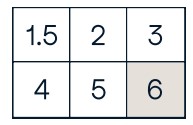
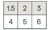
my_2darray = np.array([[1,2,3],[4,5,6]])
Selecting Numpy Array Elements
Index starts at 0
Subset
 my_array[1] #Select item at index 1
2
Slice
 my_array[ 0:2]#Select items at index 0 and 1
array([1, 2])
Subset 2D Numpy arrays
 my_2darray[:,0]#my_2darroy[rows, columns]
array([1, 4])
Numpy Array Operations
 my_array > 3
array([False, False, False, True], dtype=bool)
 my_array *  2
array([2, 4, 6, 8])
 my_array + np.array([5, 6, 7, 8])
array([6, 8, 10, 12])
Numpy Array Functions
 my_array.shape #Get the dimensions of the array
 np.append(other_array) #Append items to on array
 np.insert( my_array, 1, 5) #Insert items in on array
 np.delete( my_array,[1]) #Delete items in on array
 np.mean(my_array) #Mean of the array
 np.median(my_array) #Median of the array
 my_array.corrcoef() #Correlation coefficient
 np.std( my_array) #Standard deviation
Lists
 a  =  'is'
 b  =  'nice'
 my_list = ['my','list', a, b]
 my_list2=[[4,5,6,7],[3,4,5,6]]
Selecting List Elements
Index starts at 0
Subset
 my_list[1] #Select item at index 1
 my_list[-3] #Select 3rd last item
Slice
 my_list[1:3] #Select items at index 1 and 2
 my_list[1:] #Select items after index 0
 my_list[:3] #Select items before index 3
 my_list[:] #Copy my_list
Subset Lists of Lists
 my_list2[1][0] #my_list[list][itemOfList]
 my_list2[1][:2]
List Operations
 my_list + my_list
    ['my','list','is','nice','my','list','is','nice']
 2*my_list
    ['my','list','is','nice','my','list','is','nice']
List Methods
 my_list.index(a) #Get the index of an item
2
 my_list.count(a) #Count on item
1
 my_list.append( '!') #Append on item ot a time
['my','list','is','nice','!']
 my_list.remove( '!' ) #Remove  on  item
 del(my_list[0:1]) #Remove an item
['list','is','nice']
 my_list.reverse() #Reverse the list
['nice','is','list','my']
 my_list.extend('!') #Append on item
 my_list.pop(-1) #Remove on item
 my_list.insert(0, '!') #Insert on item
 my_list.sort() #Sort the list
Asking For Help
help(str)
Section 2
Importing Data
Most of the time, you’ll use either NumPy or pandas to import your data:
 import numpy as np
 import pandas as pd
Help
 np.info(np.ndarray.dtype)
 help(pd.read_csv)
Text Files
Plain Text Files
filename= 'huck_finn.txt'
file= open(filename, mode= 'r' ) #Open the file for reading
text= file.read() #Reado file's contents
 print(file.closed) #Check whether file is closed
 file.close() #Close file
 print(text)
 with open('huck_finn.txt', 'r' ) as file:
    print(file.readline()) #Read single line
    print(file.readline())
    print(file.readline())
Table Data: Flat Files
Importing Flat Files with NumPy
filename= 'huck_finn.txt'
file= open(filename, mode= 'r' ) #Open the file for reading
text= file.read() #Reado file's contents
 print(file.closed) #Check whether file is closed
 file.close() #Close file
 print(text)
Files with one data type
filename= 'mnist.txt'
data= np.loadtxt(filename,
					delimiter=',' , #String used to separate values
                    skiprows=2, #Skip the first 2 lines
                    usecols=[0,2], #Read the 1st and 3rd column
                    dtype=str) #The type of the resulting array
Files with mixed data type
filename= 'titanic.csv'
data= np.genfromtxt(	filename,
					   	delimiter = ',',
					   	names=True, #Look for column header
						dtype=None)
 data_array = np.recfromcsv(filename)
#The default dtype of the np.recfromcsv() function is None
Importing Flat Files with Pandas
filename= 'winequality-red.csv'
data= pd.read_csv(filename,
					 nrows=5, #Number of rows of file to read
                     header=None, #Row number to use as col names
                     sep='\t', #Delimiter to use
					 comment='#', #Character to split comments
					 na _values=[""]) #String to recognize as NA/NaN
Exploring Your Data
NumPy Arrays
 data_array.dtype #Data type of array elements
 data_array.shape #Array dimensions
 len(data_array) #Length of array
Pandas DataFrames
 df.head() #Return first DataFrame rows
 df.tail() #Return last OataFrame rows
 df.index #Describe index
 df.columns #Describe OataFrame columns
 df.info() #Info an DataFrame
 data_array = data.values #Convert a DataFrame to an a NumPy array
SAS File
 from sas7bdat import SAS7BDAT
 with SAS7BDAT( 'urbanpop .sas7bdat') as file:
		df_sas = file.to_da ta_frame()
Stata File
data= pd.read_stata('urbanpop .dta')
Excel Spreadsheets
file= 'urbanpop.xlsx'
data= pd.ExcelFile(file)
 df_sheet2 = data.parse('1960-1966',
				skiprows=[0], names=['Country',
					'AAM: War(2002)'])
 df_sheetl = data.parse(0,
				parse_cols=[0], skiprows=[0],
				name s=['Country'])
To access the sheet names, use the sheet_names attribute:
data.sheet_names
Relational Databases
 from sqlalchemy import create _engine
engine= create_engine('sq lite://Northwind.sqlite')
Use the table_name s() method to fetch a list of table names:
table_names = engine.table_names()
Querying Relational Databases
con= engine.connect()
 rs= con.execute('SELECT* FROM Order s')
 df = pd.DataFrame(rs.fetchall())
 df.columns = rs.keys()
 con.close()
Using the context manager with
 with engine.connect() as con:
rs= con.execute('SELEC T OrderID FROM Order s')
                df = pd.DataFrame(rs.fetchmany(size=5))
                df.columns = rs.keys()
Querying relational databases with pandas
df = pd.read_sql_query( ''SELECT* FROM Orders'', engine)
Pickled File
 import pickle
 with open('pickled_fruit.pkl', 'rb' ) as file: pickled_data = pickle.load(file)
Matlab File
 import scipy.io
filename= 1 workspace.m at 1
mat= scipy.io.loadmat(filename)
HDF5 Files
 import h5py
filename= 'file.hdf5'
data= h5py.File(filename, 'r' )
Exploring Dictionaries
Querying relational databases with pandas
 print(mat.keys()) #Print dictionary keys
 for key in data.keys(): #Print dictionary keys
print(key)
meta quality strain
 pickled_data.values() #Return dictionary values
 print(mat.items()) #Returns items in list format of (key, value) tuple pairs
Accessing Data Items with Keys
 for key in data['meta'].keys() #Explore the HOF5
structure
print(key) Description DescriptionURL Detector
Duration GPSstart Observatory Type UTCstart
#Retrieve the value for a key
 print(data['meta']['Description'].value)
Navigating Your FileSystem
Magic Commands
!ls #List directory contents of files and directories
%cd .. #Change current working directory
%pwd #Return the current working directory path
OS Library
 import os
 path = "/usr/tmp"
 wd = os.getcwd() #Store the name of current directory in a string
 os.listdir(wd) #Output contents of the directory in a list
 os.chdir(path) #Change current working directory
 os.rename( "testl.txt", #Rename a file
 				"test2.txt" )
 os.remove( "test1. txt") #Oelete an existing file
 os.mkdir( "newdir") #Create a new directory
Pivot
 df3= df2.pivot(inde x='Date', #Spread rows into columns
col umns= 'Type' ,
values='Value' )
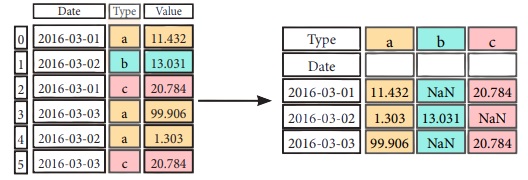
Pivot Table
 df4 = pd.pivot_table(df2, #Spread rows into
columns values='Value', index='Date', columns='Type'])
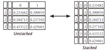
Stack / Unstack
stacked= df5.stack() #Pivot o level of column labels
 stacked.unstack() #Pivot o level of index labels
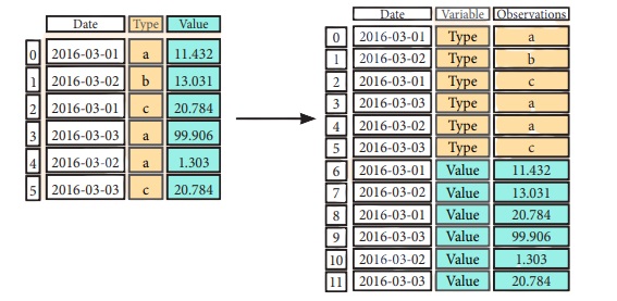
Melt
 pd.melt(df2, #Gather columns into rows
		id _vars=[°Date°],
		value_var s=['Type','Value'],
		value name=''Observations'')
Iteration
 df.iteritems() #{Column-index, Series) pairs
 df.iterrows() #{Row-index, Series) pairs
Missing Data
 df.dropna() #Drop NaN values
 df3.fillna(df3.mean()) #Fill NaN values with o predetermined value
 df2.replace("a" , "f") #Replace values with others
Advanced Indexing
Selecting
 df3.loc[:,(df3>1).any()] #Select cols with any vols >1
 df3.loc[:,(df3>1).all()] #Select cols with vols> 1
 df3.loc[:,df3.isnull().any()] #Select cols with NaN
 df3.loc[:,df3.notnull().all()] #Select cols without NaN
Indexing With isin ()
 df[(df.Country.isin(df2.Type))] #Find some elements
 df3.filter(iterns="a","b"]) #Filter on values
 df.select(lambda x: not x%5) #Select specific elements
Where
s.where(s > 0) #Subset the data
Query
df6.query('second > first') #Query DataFrame
Setting/Resetting Index
 df.set_index('Country' ) #Set the index
 df4 = df.reset_index() #Reset the index
 df = df.rename(index=str, #Rename
			DataFrame columns={	"Country":"cntry",
								"Capital':"cptl",
								"Population":pplt})
Reindexing
s2=s.reindex(['a','c','d','e','b'])
Forward Filling
 df.reindex(	range(4),
				method= 'ffill')
	Country	Capital		Population
0	Belgium	Brussels	11190846
1	India	New Delhi	1303171035
2	Brazil	Brasilia	207847528
3	Brazil	Brasilia	207847528
Backward Filling
 s3 = s.reindex(	range(5),
					method= 'bfill')
0	3
1	3
2	3
3	3
4	3
Multilndexing
arrays= [np.array([l,2,3]),
np.array([5,4,3])]
 df5 = pd.DataFrame(np.random.rand(3, 2), index=arrays)
tuples= list(zip(*arrays))
index= pd.Multilndex.from_tuples(tuples,
names= [ 'first' , 'second' ])
 df6 = pd.DataFrame(np.random.rand(3, 2), index=index)
 df2.set_index([ "Date", "Type"])
Duplicate Data
 s3.unique() #Return unique values
 df2.duplicated('Type') #Check duplicates
 df2.drop_dup licates( 'Type', keep='last') #Drop duplicates
 df.index.duplicated() #Check index duplicates
Grouping Data
Aggregation
 df2.groupby(by=['Date','Type']).mean()
 df4.groupby(level=0).sum()
 df4.groupby(level=0).agg({ 'a':lambda x:sum(x)/len (x), 'b': np.sum})
Transformation
 customSum = lambda x: (x+x%2)
 df4.groupby(level=0).transform(customSum)
Combining Data
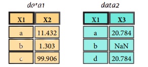
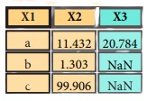
Merge
 pd.merge(data1,
            data2,
            how = 'left' ,
            on='X1')
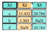
 pd.merge(data1,
            data2,
            how = 'right' ,
            on='X1')
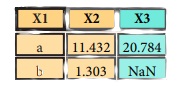
 pd.merge(data1,
            data2,
            how='inner',
            on='X1')
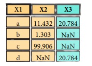
 pd.merge(data1,
			data2,
             how='outer',
             on='X1')
Join
datal.join(data2, ho w='righ t')
Concatenate
Vertical
s.append(s2)
Horizontal/Vertical
 pd.concat([s,s2],axis=l, keys=['One' ,'Two'])
 pd.concat([data1, data2], axis=l, join='inner')
Dates
 df2['Date']= pd.to_da tetime(d f2['Date'])
 df2['Date']= pd.da te_range( '2000-1-1',
periods=6, freq='M' )
dates= [datetime(2012,5,1), datetime(2012,5,2)]
index= pd.Datetimelndex(dates)
index= pd.date_range(datetime(2012,2,1), end, freq='BM' )
Visualization
 import matplotlib.pyplot as plt
 s.plot()
 plt.show()
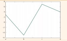
df2.plot()
 plt.show()
Section 3
Data Wrangling with Pandas

The Pandas library is built on NumPy and provides easy-to-use data structures and data analysis tools for the Python programming language.
Use the following import convention:
import pandas as pd
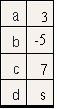
Pandas Data Structure
Series
A one-dimensional labeled array
capable of holding any data type
s = pd.Series([3,-5,7, s], index=['a','b','c','d'])
Dataframe
A two-dimensional labeled data structure with columns of potentially different types
 data = { 'Country' : ['Belgium' ,'India ',' Brazil'  ] ,
			  'Capital': ['Brussels','New Delhi','Brasilia'] ,
			'Population': [111908s6, 1303171035, 207847528]}
 df = pd.DataFrame(data,columns=[ 'Country' , 'Capital' , 'Population' ])
Dropping
 s.drop(['a', 'c']) #Drop values from rows (axis=B)
 df.drop( 'Country', axis=l) #Drop values from columns(axis=l)
Sort & Rank
 df.sort_index() #Sort by labels along an axis
 df.sort_values( by='Country') #Sort by the values along on axis
 df.rank() #Assign ranks to entries
I/O
Read and Write to CSV
 pd.read_csv('file.csv', header=None, nrows=5)
 df.to_csv('myDataFrame.csv')
Read and Write to Excel
 pd.read_excel( 'file.xlsx')
 df.to_excel('dir/myDataFrame.x lsx', sheet_name= 'Sheet1')
Read multiple sheets from the same file
 xlsx = pd.ExcelFile('file.xls')
 df = pd.read_excel(xlsx, 'Sheet1')
Read and Write to SQL Query or Database Table
 from sqlalchemy import create_engine
 engine = create_eng ine('sqlite:///:memory:' )
 pd.read_sql( "SELECT* FROM my_tabl e;", engine)
 pd.read_sql_ tabl e('my_ tabl e', engine)
 pd.read_sql_query( "SELECT * FROM my_table;", engine)
read_sql() is a convenience wrapper around read_sql_table() and read_sql_query()
df.to_sql('myDf',engine)
Selection
Getting
 s['b'] #Get one element
-5
 df[l:] #Get subset of a DataFrome
Country Capital Population 1 India New Delhi 1303171035
2 Brazil Brasilia 207847528
Selecting, Boolean Indexing & Setting
By Position
 df.iloc[[0],[0]] #Select single value by row & column
'Belgium'
 df.iat([0],[0])
'Belgium'
By Label
 df.loc[[0], [ 'Country']] #Select single value by row & column labels 'Belgium'
 df.at([0], [ 'Country ']) 'Belgium'
By Label/Position
 df.ix[2] #Select single row of subset of rows
Country Brazil Capital Brasilia Population 207847528
 df.ix[:,'Capital'] #Select a single column of subset of columns
0	Brussels
1	New Delhi
2	Brasilia
 df.ix[1,'Capital'] #Select rows and columns 'New Delhi'
Boolean Indexing
 s[N(s > 1)] #Series s where value is not >l
 s[(s < -1) I (s > 2)] #s where value is f-1 or >2
 df[df['Population']>1200000000] #Use filter to adjust DataFrame
Setting
s['a'] = 6 #Set index a of Series s to 6
Retrieving Series/DataFrame Information
Basic Information
 df.shape #(rows,columns)
 df.index #Describe index
 df.columns #Describe DataFrame columns
 df.info() #Info on DataFrame
 df.count() #Number of non-NA values
Summary
 df.sum() #Sum of values
 df.cumsum() #Cummulative sum of values
 df.min() /df.max() #11inimum/maximum values
 df.idxmin()/df.idxmax() #Minimum/Maximum index value
 df.describe() #Summary statistics
 df.mean() #11ean of values
 df.median() #Median of values
Applying Functions
 f = lambda x: X*2
 df.apply(f) #Apply function
 df.applymap(f) #Apply function element-wise
Data Alignment
Internal Data Alignment
 s3 = pd.Series([7, -2, 31, index= ['a','c' ,'d'])
 s + s3
a 10.0
b NaN
C 5.0
d 7.0
Arithmetic Operations with Fill Methods
You can also do the internal data alignment yourself with the help of the fill methods:
 s.add(s3, fill_values=0) a 10.0
b -5. 0
C 5.0
d 7.0
 s.sub(s3, fill_value=2)
 s.div(s3, fill_value=4)
 s.mul(s3, fill_value=3)
Section 4
Data Analysis with Numpy

The NumPy library is the core library for scientific computing in Python. It provides a high performance multidimensional array object , and tools for working with these arrays
Use the following import convention
import numpy as np
Creating Array
 a = np.array([l,2,3])
 b = np.array([(l.5,2,3), (4,5,6)], dtype = float)
 c = np.array([[(l.5,2,3), (4,5,6)],[(3,2,1), (4,5,6)]], dtype = float)
Initial Placeholders
 np.zeros((3,4)) #Create an array af zeros
 np.ones((2,3,4),dtype=np.int16) #Create an array of ones
 d = np.arange(10,25,5) #Create an array of evenly spaced values (step value)
 np.linspace(0,2,9) #Create an array of evenly spaced values (number of samples)
 e = np.full((2,2),7) #Create a constant array
 f = np.eye(2) #Create a 2X2 identity matrix
 np.random.random((2,2)) #Create an array with random values
 np.empty((3,2)) #Create an empty array
I/O
Saving & Loading On Disk
 np.save('my_array',a)
 np.save('array.npz',a, b)
 np.load('my_array.npy ')
Saving & Loading Text Files
 np.loadtxt("myfile.txt")
 np.genfromtxt("my_file.csv", delimiter=',' )
 np.savetxt("myarray.txt" , a, delimiter=" " )
Inspecting Your Array
 a.shape #Array dimensions
 len(a) #Length of array
 b.ndim #Number of array dimensions
 e.size #Number of array elements
 b.dtype #Data type of array elements
 b.dtype.name #Name of data type
 b.astype(int) #Convert an array to a different type
Data Type
 np.int64 #Signed 64-bit integer types
 np.flaat32 #Standard double-precision floating paint
 np.complex #Complex numbers represented by 128 floats
 np.baol #Boolean type storing TRUE and FALSE values
 np.object #Python object type
 np.string _ #Fixed-length string type
 np.unicode_ #Fixed-length unicode type
Array Mathematics
Arithmetic Operations
 g = a - b #Subtraction
array([[-0.5,0. , 0. ],
		[-3. , -3. , -3. ]])
 np.subtract(a,b) #Subtraction
 b + a #Addition
array([[ 2.5, 4. , 6. ],
		[5.,7.,9.]])
 np.add(b,a) Addition
 a / b #Division
array([[ 0.66666667, 1., 1.],
		[ 0.25 , 0.4 , 0.5 ]])
 np.divide(a,b) #Division
 a * b #Multiplication
array([[ 1.5, 4. , 9. ],
	[ 4. , 10. , 18. ]])
 np.multiply(a,b) #Multiplication
 np.exp(b) #Exponentiation
 np.sqrt(b) #Square root
 np.sin(a) #Print sines of an array
 np.cos(b) #Element-wise cosine
 np.log(a) #Element-wise natural logarithm
 e.dot(f) #Dot product
array([[ 7., 7.],
Comparison
a == b #Element-wise comparison
array([[False, True , True],
[ False, False, False]], dtype=bool)
 a < 2 #Element-wise comparison
array([True , False, False], dtype=bool)
 np.array_equal(a, b) #Array-wise comparison
Aggregate Functions
 a.sum() #Array-wise sum
 a.min() #Array-wise minimum value
 b.max(axis=0) #Maximum value of an array row
 b.cumsum(axis=l) #Cumulative sum of the elements
 a.mean() #Mean
 b.median() #Median
 a.corrcaef() #Correlation coefficient
 np.std(b) #Standard deviation
Copying Array
 h = a.view() #Create a view af the array with the some data
 np.capy(a) #Create a copy of the array
 h = a.copy() #Create a deep copy of the array
Sorting Array
Subsetting
 a[2] #Select the element at the 2nd index
3
 b[1,2] #Select the element at row 1 column 2 (equivalent to b[1][2])
6.0
Slicing
 a[0:2] #Select items at index 0 and 1
array([1, 2])
 b[0:2,1] #Select items at rows 0 and 1 in column 1
array([ 2., 5.])
 b[:1] #Select all items at row 0 (equivalent to b[0:1, :])
array([[1.5, 2., 3.]])
 c[1,... ] #Same as [1,:,:]
array([[[ 3., 2., 1.],
[  4., 5.,	6.]]])
 a[: :-1] #Reversed array a array([3, 2, 1])
Boolean Indexing
 a[a<2] #Select elements from a less than 2
array([1])
Fancy Indexing
 b[[l, 0, 1, 0],[0, 1, 2, 0]] #Select elements (1,0),(0,1),(1,2) and (0,0)
array([ 4. , 2. , 6. , 1.5])
 b[[l, 0, 1, 0]][:,[0,1,2,0]] #Select a subset of the matrix's rows and columns array([[ 4. ,5. , 6. , 4. ],
            [ 1.5, 2.3,	1.5],
Array Manipulation
Transposing Array
 i = np.transpose(b) #Permute array dimensions
 i.T #Permute array dimensions
Changing Array Shape
 b.ravel() #Flatten the array
 g.reshape(3,-2) #Reshape, but don't change data
Adding/Removing Elements
 h.resize((2,6)) #Return a new array with shape (2,6)
 np.append(h,g) #Append items to an array
 np.insert(a, 1, 5) #Insert items in an array
 np.delete(a,[1]) #Delete items from an array
Combining Arrays
 np.concatenate((a,d),axis=0) #Concatenate arrays array([ 1, 2, 3, 10, 15, 20])
 np.vstack((a,b)) #Stack arrays vertically (row-wise)
array([[ 1. , 2.	3. ],
        [ 1.5, 2. , 3. ],
        [   4.    ,   5.    ,   6.    ]])
 np.r_[e,f] #Stack arrays vertically (row -wise)
 np.hstack((e,f)) #Stack arrays horizontally (col umn-wise)
array([[ 7., 7., 1., 0.],
    [ 7., 7., 0., 1.]])
 np.column_stack((a,d)) #Create stacked column-wise arrays
array([[ 1, 10],
    [ 2,  15],
    [ 3, 20]])
 np.c_[a ,d] #Create stacked column-wise arrays
Splitting Arrays
 np.hsplit(a,3) #Split the array horizontally at the 3rd index
[array([1]),array([2]),array([3])]
 np.vsplit(c,2) #Split the array vertically at the 2nd index
[array([[[ 1.5, 2. , 1. ],
        [ 4. , 5. , 6. ]]]),
array([[[ 3., 2., 3.],
        [  4.,	5.,	6.]]])]
Section 5
Data Visualization with Matplotlib
Matplotlib is a Python 2D plotting library which produces publication-quality figures in a variety of hardcopy formats and interactive environments across platforms.
1D Data
 import numpy as np
 X = np.linspace(0, 10, 100)
 y = np.cos(x)
 z = np.sin(x)
2D Data or Images
 data= 2 * np.random.random((10, 10))
 data2 = 3 * np.random.random((10, 10))
 Y, X = np.mgrid[-3:3:100j, -3:3:100j]
 U = -1 - X**2 + Y
 V = 1 +  X - Y**2
 from matplotlib.cbook import get_sample_data
 img = np.load(g et_sample_data('axes_gr id/bivar iate_normal.npy '))
Create Plot
import matplotlib.pyplot as plt
Figure
 fig = plt.figure()
 fig2 = plt.figure(figsize=plt.figaspect(2.0))
Axes
ll plotting is done with respect to an Axes. In most cases, a subplot will fit your needs. A subplot is an axes on a grid system.
 fig.add_axes()
 ax1 = fig.add_subplot(221)#row-col-num
 ax3 = fig.add_subplot(212)
 fig3, axes= plt.subplots(nrows=2,ncols=2)
 fig4, axes2 = plt.subplots(ncols=3)
Save Plot
 plt.savefig( 'foe.png' J #Save figures
 plt.savefig( 'foo.png',transparent=True) #Save transparent figures
Show Plot
plt.show()
Plotting Routines
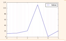
1D Data
 fig, ax= plt.subp lots()
lines= ax.plot(x,y) #Draw points with lines or markers connecting them
 ax.scatter(x,y) #Draw unconnected points, scaled or colored
 axes[0,0].bar([l,2,3],[3,4,5]) #Plot vertical rectangles (constant width)
 axes[l,0].barh([0.5,1,2.5],[0,1,2]) #Plot horiontol rectangles (constant height)
 axes[l,1].axhline(0.s5) #Draw a horizontal line across axes
 axes[0,1].axvline(0.65) #Draw a vertical line across axes
 ax.fill(x,y,color='blue') #Drow filled polygons
 ax.fill_between(x,y,color='yellow') #Fill between y-values and 0
2D Data
 fig, ax= plt.subplots()
 im = ax.imshow(img, #Colormapped or RGB arrays
            cmap= 1 gist_ear th 1 ,
            interpolation= 1 neare st',
            vmin=-2,
            vmax =2)
 axes2[0].pcolor(data2) #Pseudocolor plot of 2D array
 axes2[0].pcolormesh(data) #Pseudocolor plot of 2D array
CS= plt.contour(Y,X,U) #Plot contours
 axes2[2].contourf(datal) #Plot filled contours
 axes2[2]= ax.clabel(CS) #Lobel a contour plot
Vector Fields
 axes[0,1].arrow(0,0,0.5,0.5) #Add an arrow to the axes
 axes[l,l].quiver(y,z) #Plot a 2D field of arrows
 axes[0,1].streamplot(X,Y,U,V) #Plot a 2D field of arrows
Data Distributions
 axl.hist(y) #Plot a histogram
 ax3.boxplot(y) #Make a box and whisker plot
 ax3.violinplot(z) #Make a violin plot
Plot Anatomy
The basic steps to creating plots with matplotlib are:
1 Prepare Data 2 Create Plot 3 Plot 4 Customized Plot 5 Save Plot 6 Show Plot
 import matplotlib.pyplot as plt
 x = [1,2,3,s] #Step 1
 y = [ 10,20,25,30]
fig= plt.figure() #Step 2
ax= fig.add_subp lot(lll) #Step 3
 ax.plot(x, y, color='lightb lue', linewidth=3) #Step 3, 4
 ax.scatter([2,4,6],
                [5,15,25],
                color='darkgreen ',
                marker='^')
 ax.set_xlim(l, 6.5)
 plt.savefig('foo.png' ) #Step 5
 plt.show() #Step 6
Close and Clear
 plt.cla() #Clear on axis
 plt.clf() #Clear the entire figure
 plt.close() #Close a window
Plotting Cutomize Plot
Colors, Color Bars & Color Map
 plt.plot(x, x, x, X**2, x, X**3)
 ax.plot(x, y, alpha = 0.s)
 ax.plot(x, y, c='k' )
 fig.colorbar(im, orientation= 'horizontal')
 im = ax.imshow(img,cmap=  'seismic'  )
Markers
 fig, ax= plt.subplots()
 ax.scatter(x,y,marker="."   )
 ax.plot(x,y ,marker="o")
Linestyles
 plt.plot(x,y,linewidth=4.0)
 plt.plot(x,y,ls='solid')
 plt.plot(x,y,ls='--' )
 plt.plot(x, y,'-- 1 ,X**2,Y** 2, '-.')
 plt.setp(lines,color='r',linewidth= 4.0)
Text & Annotations
 ax.text(1,-2.1,'Example Graph' , style='italic')
 ax.annotate("Sine",
                xy=(8, 0),
                xycoords= 'data',
                xytext=(10.5, 0),
                textcoords= 1 data',
                arrowprops=dict(arrowstyle= "->" connectionstyle="arc3"),)
Mathtext
plt.title(r'$sigma_ i=15$', fontsize=20)
Limits, Legends and Layouts
Limits & Autoscaling
 ax.margins(x=0.0,y=0.1) #Add padding to a plot
 ax.axis('equa l') #Set the aspect ratio of the plot to 1
 ax.set(xlim=[0,10.5],ylim=[-1.5,l.5]) #Set limits for x-and y-axis
 ax.set_xlim(0,10.5) #Set limits for x-axis
Legends
 ax.set(	title='An Example Axe s', #Set a title and x-ond y-axis labels
           ylabel='Y-Axis',
           xlabel='X-Axis')
 ax.legend( loc='best') #No overlapping plot elements
Ticks
 ax.xaxis.set(ticks=range(l,5), #Manually set x-ticks
ticklabels=[3,100,-12,"foo']')
     #Makey-ticks longer and go in and out
 ax.tick_param s(axis='y',direction='inout ',length=10)
Subplot Spacing
 fig3.subplots_ad just(wspace=0.5, #Adjust the spacing between subplots
hspace=0.3, left=0.125, right=0.9, top=0.9, bottom=0.1)
 fig.tight_layout() #Fit subplot(s) in to the figure area
Axis Spines
 axl.spines['top'].set_visible(False)
#Make the top axis line for a plot invisible
 axl.spines['bottom'].set_po sition(('outward' ,10))
#Move the bottom axis line outward
Section 6
Queries in SQL

Querying data from a table
Query data in columns c1, c2 from a table
SELECT c1, c2 FROM t;
Query all rows and columns from a table
SELECT * FROM t;
Query data and filter rows with a condition
SELECT c1, c2 FROM t
WHERE condition;
Query distinct rows from a table
SELECT DISTINCT c1 FROM t
WHERE condition;
Sort the result set in ascending or descending order
SELECT c1, c2 FROM t
ORDER BY c1 ASC [DESC];
Skip offset of rows and return the next n rows
SELECT c1, c2 FROM t
ORDER BY c1
LIMIT n OFFSET offset;
Group rows using an aggregate function
SELECT c1, aggregate(c2)
FROM t
GROUP BY c1;
Filter groups using HAVING clause
SELECT c1, aggregate(c2)
FROM t
GROUP BY c1
HAVING condition;
Querying from multiple tables
Inner join t1 and t2
SELECT c1, c2
FROM t1
INNER JOIN t2 ON condition;
Left join t1 and t1
SELECT c1, c2
FROM t1
LEFT JOIN t2 ON condition;
Right join t1 and t2
SELECT c1, c2
FROM t1
RIGHT JOIN t2 ON condition;
Perform full outer join
SELECT c1, c2
FROM t1
FULL OUTER JOIN t2 ON condition;
Produce a Cartesian product of rows in tables
SELECT c1, c2
FROM t1
CROSS JOIN t2;
Another way to perform cross join
SELECT c1, c2
FROM t1, t2;
Join t1 to itself using INNER JOIN clause
SELECT c1, c2
FROM t1 A
INNER JOIN t1 B ON condition;
Using SQL Operators
Combine rows from two queries
SELECT c1, c2 FROM t1
UNION [ALL]
SELECT c1, c2 FROM t2;
Return the intersection of two queries
SELECT c1, c2 FROM t1
INTERSECT
SELECT c1, c2 FROM t2;
Subtract a result set from another result set
SELECT c1, c2 FROM t1
MINUS
SELECT c1, c2 FROM t2;
Query rows using pattern matching %, _
SELECT c1, c2 FROM t1
WHERE c1 [NOT] LIKE pattern;
Query rows in a list
SELECT c1, c2 FROM t
WHERE c1 [NOT] IN value_list;
Query rows between two values
SELECT c1, c2 FROM t
WHERE  c1 BETWEEN low AND high;
Check if values in a table is NULL or not
SELECT c1, c2 FROM t
WHERE  c1 IS [NOT] NULL;
Managing tables
Create a new table with three columns
CREATE TABLE t (
     id INT PRIMARY KEY,
     name VARCHAR NOT NULL,
     price INT DEFAULT 0
);
Delete the table from the database
DROP TABLE t ;
Add a new column to the table
ALTER TABLE t ADD column;
Drop column c from the table
ALTER TABLE t DROP COLUMN c ;
Add a constraint
ALTER TABLE t ADD constraint;
Drop a constraint
ALTER TABLE t DROP constraint;
Rename a table from t1 to t2
ALTER TABLE t1 RENAME TO t2;
Rename column c1 to c2
ALTER TABLE t1 RENAME c1 TO c2 ;
Remove all data in a table
TRUNCATE TABLE t;
Using SQL constraints
Set c1 and c2 as a primary key
CREATE TABLE t(
    c1 INT, c2 INT, c3 VARCHAR,
    PRIMARY KEY (c1,c2)
);
Set c2 column as a foreign key
CREATE TABLE t1(
    c1 INT PRIMARY KEY,
    c2 INT,
    FOREIGN KEY (c2) REFERENCES t2(c2)
);
Make the values in c1 and c2 unique
CREATE TABLE t(
    c1 INT, c1 INT,
    UNIQUE(c2,c3)
);
Ensure c1 > 0 and values in c1 >= c2
CREATE TABLE t(
  c1 INT, c2 INT,
  CHECK(c1> 0 AND c1 >= c2)
);
Set values in c2 column not NULL
CREATE TABLE t(
     c1 INT PRIMARY KEY,
     c2 VARCHAR NOT NULL
);
Modifying Data
Insert one row into a table
INSERT INTO t(column_list)
VALUES(value_list);
Insert multiple rows into a table
INSERT INTO t(column_list)
VALUES (value_list),
       (value_list), …;
Insert rows from t2 into t1
INSERT INTO t1(column_list)
SELECT column_list
FROM t2;
Update new value in the column c1 for all rows
UPDATE t
SET c1 = new_value;
Update values in the column c1, c2 that match the condition
UPDATE t
SET c1 = new_value,
        c2 = new_value
WHERE condition;
Delete all data in a table
DELETE FROM t;
Delete subset of rows in a table
DELETE FROM t
WHERE condition;
Managing Views
Create a new view that consists of c1 and c2
CREATE VIEW v(c1,c2)
AS
SELECT c1, c2
FROM t;
Create a new view with check option
CREATE VIEW v(c1,c2)
AS
SELECT c1, c2
FROM t;
WITH [CASCADED | LOCAL] CHECK OPTION;
Create a recursive view
CREATE RECURSIVE VIEW v
AS
select-statement -- anchor part
UNION [ALL]
select-statement; -- recursive part
Create a temporary view
CREATE TEMPORARY VIEW v
AS
SELECT c1, c2
FROM t;
Delete a view
DROP VIEW view_name;
Managing indexes
Create an index on c1 and c2 of the t table
CREATE INDEX idx_name
ON t(c1,c2);
Create a unique index on c3, c4 of the t table
CREATE UNIQUE INDEX idx_name
ON t(c3,c4)
Drop an index
DROP INDEX idx_name;
Managing triggers
Create or modify a trigger
CREATE OR MODIFY TRIGGER trigger_name
WHEN EVENT
ON table_name TRIGGER_TYPE
EXECUTE stored_procedure;
WHEN
- BEFORE – invoke before the event occurs
- AFTER – invoke after the event occurs
EVENT
- INSERT – invoke for INSERT
- UPDATE – invoke for UPDATE
- DELETE – invoke for DELETE
TRIGGER_TYPE
- FOR EACH ROW
- FOR EACH STATEMENT
Delete a specific trigger
DROP TRIGGER trigger_name;
Section 7
Machine Learning with Scikit-Learn

Scikit-learn is an open source Python library that implements a range of machine learning, preprocessing, cross-validation and visualization algorithms using a unified interface.
Example
 from sklearn import neighbors, datasets, preprocessing
 from sklearn.model_selection import train_test_split
 from sklearn.metrics import accuracy_score
iris= datasets.load_iris()
 X, y = iris.data[:, :2], iris.target
 X_train, X_test, y_train, y_test = train_test_split(X, y, random_state=33)
scaler= preprocessing.StandardScaler().fit(X_train)
 X_train = scaler.transform(X_train)
 X_test = scaler.transform(X_test)
 knn = neighbors.KNeighborsClassifier(n_neighbors=5)
 knn.fit(X_train, y_train)
 y_pred = knn.predict(X_test)
 accuracy_score(y _test, y_pred)
Loading The Data
Your data needs to be numeric and stored as NumPy arrays or SciPy sparse matrices. Other types that are convertible to numeric arrays, such as Pandas DataFrame, are also acceptable
 import numpy as np
 X = np.random.random((10,5))
 Y = np. array (['M', 'M' ,'F','F','M','F','M','M','F','F','F'])
 X[X < 0.7] = 0
Training And Test Data
 from sklearn.model_selection import train_test_split
 X_train, X_test, y_train, y_test = train_test_split(X,y, random_state=0)
Model Fitting
Supervised learning
 lr.fit(X, y) #Fit the model to the data
 knn.fit(X_train, y_train)
 svc.fit(X_train, y_train)
Unsupervised Learning
 k_mean s.fit(X_train) #Fit the model to the data
 pca_model = pca.fit_transform(X_train) #Fit to data, then transform it
Prediction
Supervised Estimators
 y_pred = svc.predict(np.random.random((2,5))) #Predict labels
 y_pred = lr.predict(X_test) #Predict labels
 y_ pred = knn.predict_proba(X_test) #Estimate probability of a label
Unsupervised Estimators
y_pred = k_means.predict(X_test) #Predict labels in clustering algos
Preprocessing The Data
Standardization
 from sklearn.preprocessing import StandardScaler
 scaler= StandardScaler().fit(X_train)
 standardized_X = scaler.transform(X_train)
 standardized_X_test= scaler.transform(X _test)
Normalization
 from sklearn.preprocessing import Normalizer
scaler= Normalizer().fit(X_train)
 normalized_X = scaler.transform(X _train)
 normalized_X_test = scaler.transform(X_test)
Binarization
 from sklearn.preprocessing import Binarizer
 binarizer = Binarizer(threshold=0.0).fit(X)
 binary_X = binarizer.transform(X)
Encoding Categorical Features
 from sklearn.preprocessing import LabelEncoder
enc= LabelEncoder()
 y = enc.fit_transform(y)
Imputing Missing Values
 from sklearn.preprocessing import Imputer
imp= Imputer(missing_values=0, strategy='mean ', axis=0)
 imp.fit_transform(X_train)
Generating Polynomial Features
 from sklearn.preprocessing import PolynomialFeatures
poly= PolynomialFeatures(5)
 poly.fit_transform(X)
Create Your Model
Supervised Learning Estimators
Linear Regression
 from sklearn. linear m_ odel import LinearRegression
 lr = LinearRegression(normalize=True)
Support Vector Machines (SVM)
 from sklearn.svm import SVC
SVC= SVC(kernel='linear')
Naive Bayes
 from sklearn.naive_bayes import GaussianNB
 gnb = GaussianNB()
KNN
 from sklearn import neighbors
 knn = neighbors.KNeighborsClassifier(n_neighbors=5)
Unsupervised Learning Estimators
Principal Component Analysis (PCA)
 from sklearn.decomposition import PCA
pea= PCA(n_components=0.95)
K Means
 from sklearn.cluster import KMeans
 k_means = KMeans(n_clusters=3, random_state=0)
Evaluate Your Model’s Performance
Classification Metrics
Accuracy Score
 knn.score(X_test, y_test) #Estimator score method
 from sklearn.metrics import accuracy_score #Metric scoring functions
 accuracy_score(y_test, y_pred)
Classification Report
 from sklearn.metrics import classification_report #Precision, recall, fl-score and support
 print(classification_report(y_test, y_pred))
Confusion Matrix
 from sklearn.metrics import confusion_matrix
 print(confusion_matrix(y_test.y_pred))
Regression Metrics
Mean Absolute Error
 from sklearn.metrics import mean_absolute_error
 y_true = [3, -0.5,2]
 mean_absolute_error(y_true, y_pred)
Mean Squared Error
 from sklearn.metrics import mean_squared_error
 mean_squared _error(y_test, y_ pred)
R2 Score
 from sklearn.metrics import r2_score
 r2_score(y_true, y_ pred)
Clustering Metrics
Adjusted Rand Index
 from sklearn.metrics import adjusted_rand_score
 adjusted_rand_score(y_true, y_pred)
Homogeneity
 from sklearn.metrics import homogeneity_score
 homogeneity_score(y_true, y_pred)
V-measure
 from sklearn.metrics import v_measure_score
metrics.v_measure_score(y_true , y_pred)
Cross-Validation
 from sklearn.cross_validation import cross_val_score
 print(cross_val_score(knn, X_train, y_train, cv=4))
 print(cross_val_score(lr, X, y, cv=2))
Tune Your Model
Grid Search
 from sklearn.grid_search import GridSearchCV
 params = {"n_neighbors "  : np.arange(l,3),
				"metric "	 : [ "euclidean" , "cityblock "] }
grid= GridSearchCV(estimator=knn,
					param_grid=params)
 grid.fit(X_train, y_train)
 print(grid.best_score_)
 print(grid.best_estimator_.n_neighbors)
Randomized Parameter Optimization
 from sklearn.grid _search import RandomizedSearchCV
 params = { "n_neighbors":range(l,5), "weights": ["unifomr","distance"]}
 rsearch = RandomizedSearchCV(estimator=knn, param_distributions=params,
                                cv=4, n_iter=S, random_state=5)
 rsearch.fit(X_train, y_train)
 print(rsearch.best_score_)
Section 8
SciPy

The SciPy library is one of the core packages for scientific computing that provides mathematical algorithms and convenience functions built on the NumPy extension of Python.
 import numpy as np
 a= np.array([1,2,3])
 b = np.array([(1+5j,2j,3j), (4j,5j,6j)])
 c = np.array([[(1.5,2,3), (4,5,6)], [(3,2,1), (4,5,6)]])
Index Tricks
 np.mgrid[0:5,0:5] #Create a dense meshgrid
 np.ogrid[0:2,0:2] #Create an open meshgrid
 np.r_[[3,[0]*5,-1:1:10j] #Stack arrays vertically (row-wise)
 np.c_[b,c] #Create stocked column-wise arrays
Shape Manipulation
 np.transpose(b) #Permute array dimensions
 b.flatten() #Flatten the array
 np.hstack((b,c)) #Stack arrays horizontally (column-wise)
 np.vstack((a,b)) #Stack arrays vertically (row-wise)
 np.hsplit(c,2) #Split the array horizontally at the 2nd index
 np.vpslit(d,2) #Split the array vertically at the 2nd index
Polynomials
 from numpy import polyld
 p = poly1d([3,4,5]) #Create a polynomial object
Vectorizing Functions
 def myfunc(a): if a< 0:
        return a*2
        else:
        return a/2
 np.vectorize(myfunc) #Vectorize functions
Type Handling
 np.real(c) #Return the real part of the array elements
 np.imag(c) #Return the imaginary part of the array elements
 np.real_if_close(c,tol=1000) #Return a real array if complex parts close to 0
 np.cast['f'](np.pi) #Cast object to a data type
Other Useful Functions
 np.angle(b,d eg=True) #Return the angle of the complex argument
 g = np.linspace(0,np.pi,num=5) #Create an array of evenly spaced values(number of samples)
 g [3:] += np.pi
 np.unwrap(g) #Unwrap
 np.logspace(0,10,3) #Create an array of evenly spaced values (log scale)
 np.select([c<li],[c*2]) #Return values from a list of arrays depending on conditions
 misc.factorial(a) #Factorial
 misc.comb( 10,3,exact=True) #Combine N things taken at k time
 misc.central_diff_weights(3) #Weights for Np-point central derivative
 misc.derivative(myfunc,1.0) #Find then-th derivative of a function at a point
Linear Algebra
You’ll use the linalg and sparse modules. Note that scipy. linalg contains and expands on numpy. linalg.
from scipy import linalg, sparse
Creating Matrices
 A = np.matrix(np.random.random((2,2)))
 B = np.asmatrix(b)
 C = np.mat(np.random.random((10,5)))
 D = n p.mat([[3,Ii],  [5,6]])
Basic Matrix Routines
 A.I #Inverse
 linalg.inv(A)  #Inverse
 A.T #Tranpose matrix
 A.H #Conjugate transposition
 np.trace(A) #Trace
Norm
linalg.norm(A) #Frobenius norm
linalg.norm(A,1) #Ll norm (max column sum)
linalg.norm(A,np.inf) #L inf norm (max row sum)
Rank
np.linalg.matrix_rank(C) #Matrix rank
Determinant
linalg.det(A) #Determinant
Solving linear problems
linalg.solve(A,b) #Solver for dense matrices
E = np.mat(a).T #Solver for dense matrices
linalg.lstsq(D,E) #Le ast-squares solution to linear matrix equation
Generalized inverse
linalg.pinv(C) #Compute the pseudo-inverse of a matrix (least-squares solver)
linalg. pinv2(C) #Compute the pseudo-inverse of a matrix (SVD)
Creating Sparse Matrices
F = np.eye(3, k=l) #Create a 2X2 identity matrix
G = np.mat(np.identity(2)) #Create a 2x2 identity matrix
C[C > 0.5] = 0
H = sparse.csr_matrix(C) #Compressed Sparse Row matrix
I= sparse.csc_matrix(D) #Compressed Sparse Column matrix
J = sparse.dok_matrix(A) #Dictionary Of Keys matrix
E.tadense() #Sparse matrix to full matrix
sparse.isspmatrix_csc(A)
Sparse Matrix Routines
Inverse
sparse.linalg.inv(I) #Inverse
Norm
sparse.linalg.norm(I) #Norm
Solving linear problems
sparse.linalg.spsolve(H,I) #Solver for sparse matrices
Sparse Matrix Functions
sparse.linalg.expm(I) #Sparse matrix exponential
Sparse Matrix Decompositions
la, v = sparse.linalg.eigs(F,1) #Eigenvalues and eigenvectors
sparse.linalg.svds(H, 2) #SVD
Matrix Function
Addition
np.add(A,D) #Addition
Subtraction
np.subtract(A,D) #Subtraction
Division
np.divide(A,D) #Division
Multiplication
np.multiply(D,A) #Multiplication
np.dot(A,D) #Dot product
np.vdot(A,D) #Vector dot product
np.inner(A,D) #Inner product
np.outer(A,D) #Outer product
np.tensardat(A,D) #Tensor dot product
np.kron(A,D) #Kronecker product
Exponential Functions
linalg.expm(A) #Matrix exponential
linalg.expm2(A) #Matrix exponential (Taylor Series)
linalg.expm3(D) #Matrix exponential (eigenvalue decomposition)
Logarithm Function
linalg.lagm(A) #Matrix logarithm
Trigonometric Functions
linalg.sinm(D) Matrix sine
linalg.cosm(D) Matrix cosine
linalg.tanm(A) Matrix tangent
Hyperbolic Trigonometric Functions
linalg.sinhm(D) #Hypberbolic matrix sine
linalg.coshm(D) #Hyperbolic matrix cosine
linalg.tanhm(A) #Hyperbolic matrix tangent
Matrix Sign Function
np.sigm(A) #Matrix sign function
Matrix Square Root
linalg.sqrtm(A) #Matrix square root
Arbitrary Functions
linalg.funm(A, lambda x: X*X) #Evaluate matrix function
Eigenvalues and Eigenvectors
la, v = linalg.eig(A) #Solve ordinary or generalized eigenvalue problem for square matrix
l1, l2 = la #Unpack eigenvalues
v[:,0] #First eigenvector
v[:,1] #Second eigenvector
linalg.eigvals(A) #Unpack eigenvalues
Singular Value Decomposition
U,s,Vh = linalg.svd(B) #Singular Value Decomposition (SVD)
M,N = B.shape
Sig= linalg.diagsvd(s,M,N) #Construct sigma matrix in SVD
LU Decomposition
P,L,U = linalg.lu(C) #LU Decomposition
Section 9
Neural Networks with Keras

Keras is a powerful and easy-to-use deep learning library for Theano and TensorFlow that provides a high-level neural networks API to develop and evaluate deep learning models.
A Basic Example
import numpy as np
from keras.models import Sequential
from keras.layers import Dense
data= np.random.random((1000,100))
labels= np.random.randint(2,size=(1000,1))
model= Sequential()
model.add(Dense(32,
activation='relu', input_dim=100))
model.add(Oense(1, activation='sigmoid'))
model.compile(optimizer='rmsprop' ,
loss='binary_crossentropy',
metrics=['accuracy' ])
model.fit(data,labels,epochs=10,batch_size=32)
predictions= model.predict(data)
Data
Your data needs to be stored as NumPy arrays or as a list of NumPy arrays. Ideally, you split the data in training and test sets, for which you can also resort to the train_test_split module of sklearn. cross_ validation.
Keras Data Sets
from keras.datasets import boston_housing, mnist, cifar10, imdb
(x_train,y_train),(x_test,y_test) = mnist.load _data()
(x_train2,y_train2),(x_test2,y_test2) = boston_housing.load_data()
(x_train3,y_train3),(x_test3,y_test3) = cifar10.load_data()
(x_train4,y_train4),(x_test4,y_test4) = imdb.load_data(num_words=20000)
num_classes = 10
Other
from urllib.request import urlopen
data =
np.loadtxt(urlopen( "http://archive.ics.uci.edu/ml/machine-learning-databa ses/pima-indians-dibetes/pima-indians-d iabetes.data')',delimiter=",")
X = data[:,0:8]
y = data [:,8]
Preprocessing
Sequence Padding
from keras.preprocessing import sequence
x_train4 = sequence.pad_sequences(x _train4,maxlen=80)
x test4 = sequence.pad_sequences(x_test4,maxlen=80)
One-Hot Encoding
from keras.utils import to_categorical
>>Y_train = to_categorical(y_train,num_classes)
Y_test = to_categorical(y_test,num_classes)
Y_train3 = to_categorical(y_train3,num_classes
Y_test3 = to_categorical(y_test3,num_classes)
Model Architecture
Sequential Model
from keras.models import Sequential
model= Sequential()
model2 = Sequential()
model3 = Sequential()
Multilayer Perceptron (MLP)
Binary Classification
from keras.layers import Dense
model.add(Dense(12,
input _dim=8,
kernel_initializer='uniform',
activation='relu') )
model.add(Dense(8,kernel_initialiezr='uniform',activation='relu'))
model.add(Dense(l,kernel_initialiezr='uniform',activation='sigmoid'))
Multi-Class Classification
from keras.layers import Dropout
model.add(Dense(512,activation='relu',input_shape=(784,)))
model.add(Dropout(0.2))
model.add(Dense(512,activation='relu'))
model.add(Dropout(0.2))
model.add(Dense(10,activation='softmax' ))
Regression
model.add(Dense(64,activation='relu',input_dim=train_data.shape[1]))
model.add(Dense(1))
Convolutional Neural Network (CNN)
from keras.layers import Activation,Conv2D,MaxPooling20,Flatten
model2.add(Conv20(32,(,3),padding= 'same',input _shape=x _train.shape[1:]))
model2.add(Activation('relu'))
model2.add(Conv20(32,(3,3)))
model2.add(Activation('relu'))
model2.add(MaxPooling2D( pool_size=(2,2)))
model2.add(Dropout(0.25))
model2.add(Conv20(64,(3,3), padding= 'same'))
model2.add(Activation('relu'))
model2.add(Conv20(64,(3, 3)))
model2.add(Activation('relu'))
model2.add(MaxPooling2D( pool_size=(2,2)))
model2.add(Dropout(0.25))
model2.add(Flatten())
model2.add(Dense(512))
model2.add(Activation('relu'))
model2.add(Dropout(0.5))
model2.add(Dense(num_classes))
model2.add(Activation('softmax'))
Recurrent Neural Network (RNN)
from keras.klayers import Embedding,LSTM
model3.add(Embedding(20000,128))
model3.add(LSTM(128,dropout =0.2,recurrent_dropout=0.2))
model3.add(Dense(l,activation='sigmoid'))
Prediction
model3.predict(x_test4, ba tch_size=32)
model3.predict_classes(x_test4,batch _size=32)
Train and Test Sets
from sklearn.mode l_selection import train_test_split
X_train5,X_test5,y_train5,y_test5 = train_test_split(X, y,
test_size=0.33, random_state=42)
Standardization/Normalization
from sklearn.preprocessing import StandardScaler
scaler= StandardScaler().fit(x_train2)
standa rdized_X = scaler.transform(x _train2)
standardized X test= scaler.transform(x_test2
Inspect Model
model.output_shape #Model output shape
model.summary() #Model summary representation
model.get_config() #Model configuration
model.get_weights()#List all weight tensors in the model
Compile Model
MLP: Binary Classification
model.compile(optimizer='adam' ,
loss= 'binary_crossentropy',
metrics=['accuracy'])
MLP: Multi-Class Classification
model.compile(optimizer='rmsprop',
loss='categorical_crossentropy ,
metrics=[ 'accuracy'])
MLP: Regression
model.compile(optimizer='rmsprop',
loss= 'mse,' metrics=['mae'])
Recurrent Neural Network
model3.compile(loss='binary_crossentropy ',
optimizer='adam',
metrics=['accuracy'])
Model Training
model3.fit(x_train4,
y_train4,
batch_size=32,
epochs=15,
verbose=1,
validation_data=(x_test4,y_test4))
Evaluate Your Model’s Performance
score = model3.evaluate(x_test,
y_test,
batch_size=32)
Save/ Reload Models
from keras.models import load_model
model3.save( )
my_model = load_model( )
Model Fine-tuning
Optimization Parameters
from keras.optimizers import RMSprop
opt = RMSprop(lr=0.0001, decay=1e-6)
model2.compile(loss= , 'categorical_crossentropy'
optimizer=opt,
metrics=[ 'accuracy'])
Early Stopping
from keras.callbacks import EarlyStopping
early_stopping_monitor = EarlyStopping(patience=2)
model3.fit(x_train4,
y_train4,
batch_size=32,
epochs=15,
validation_data=(x_test4,y_test4),
callbacks=[early_stopping_monitor])
Section 10
PySpark & Spark SQL

What is PySpark?
PySpark is an Apache Spark interface in Python. It is used for collaborating with Spark using APIs written in Python. It also supports Spark’s features like Spark DataFrame, Spark SQL, Spark Streaming, Spark MLlib and Spark Core.
What is PySpark SparkContext?
PySpark SparkContext is an initial entry point of the spark functionality. It also represents Spark Cluster Connection and can be used for creating the Spark RDDs (Resilient Distributed Datasets) and broadcasting the variables on the cluster.
from pyspark.sql import SparkSession
spark = SparkSession \
.builder \
.appName( ) \
.config( , ) \
.getOrCreate()
What is spark-submit?
Spark-submit is a utility to run a pyspark application job by specifying options and configurations.
spark-submit \
--master <master-url> \
--deploy-mode <deploy-mode> \
--conf <key<=<value> \
--driver-memory <value>g \
--executor-memory <value>g \
--executor-cores <number of cores> \
--jars <comma separated dependencies> \
--packages <package name> \
--py-files \
<application> <application args>
where
–master : Cluster Manager (yarn, mesos, Kubernetes, local, local(k))
–deploy-mode: Either cluster or client
–conf: We can provide runtime configurations, shuffle parameters, application configurations using –conf.
Ex: –conf spark.sql.shuffle.partitions = 300
–driver-memory : Amount of memory to allocate for a driver (Default: 1024M).
–executor-memory : Amount of memory to use for the executor process.
–executor cores : Number of CPU cores to use for the executor process.
What are RDDs in PySpark?
RDDs expand to Resilient Distributed Datasets. These are the elements that are used for running and operating on multiple nodes to perform parallel processing on a cluster. Since RDDs are suited for parallel processing, they are immutable elements. This means that once we create RDD, we cannot modify it. RDDs are also fault-tolerant which means that whenever failure happens, they can be recovered automatically. Multiple operations can be performed on RDDs to perform a certain task.
- Data Representation: RDD is a distributed collection of data elements without any schema
- Optimization: No in-built optimization engine for RDDs
- Schema: we need to define the schema manually.
- Aggregation Operation: RDD is slower than both Dataframes and Datasets to perform simple operations like grouping the data
Creation of RDD using textFile API
rdd = spark.sparkContext.textFile('practice/test')
rdd.take(5)
for i in rdd.take(5): print(i)
Get the Number of Partitions in the RDD
rdd.getNumPartitions()
Get the Number of elements in each partition
rdd.glom().map(len).collect()
Create RDD using textFile API and a defined number of partitions
rdd = spark.sparkContext.textFile('practice/test',10)
Create a RDD from a Python List
lst = [1,2,3,4,5,6,7]
rdd = spark.sparkContext.parallelize(lst)
for i in rdd.take(5) : print(i)
Create a RDD from a Python List
lst = [1,2,3,4,5,6,7]
rdd = spark.sparkContext.parallelize(lst)
for i in rdd.take(5) : print(i)
Create a RDD from local file
lst = open('/staging/test/sample.txt').read().splitlines()
lst[0:10]
rdd = spark.sparkContext.parallelize(lst)
for i in rdd.take(5) : print(i)
Create RDD from range function
lst1 = range(10)
rdd = spark.sparkContext.parallelize(lst1)
for i in rdd.take(5) : print(i)
Create RDD from a DataFrame
df=spark.createDataFrame(data=(('robert',35),('Mike',45)),schema=('name','age'))
df.printSchema()
df.show()
rdd1= df.rdd
type(rdd1)
for i in rdd1.take(2) : print(i)
What are Dataframes?
It was introduced first in Spark version 1.3 to overcome the limitations of the Spark RDD. Spark Dataframes are the distributed collection of the data points, but here, the data is organized into the named columns
- Data Representation:It is also the distributed collection organized into the named columns
- Optimization: It uses a catalyst optimizer for optimization.
- Schema: It will automatically find out the schema of the dataset.
- Aggregation Operation: It performs aggregation faster than both RDDs and Datasets.
What are Datasets?
Spark Datasets is an extension of Dataframes API with the benefits of both RDDs and the Datasets. It is fast as well as provides a type-safe interface.
- Data Representation:It is an extension of Dataframes with more features like type-safety and object-oriented interface.
- Optimization:It uses a catalyst optimizer for optimization.
- Schema: It will automatically find out the schema of the dataset.
- Aggregation Operation:Dataset is faster than RDDs but a bit slower than Dataframes.
What type of operation has Pyspark?
The operations can be of 2 types, actions and transformation.
What is Transformation in Pyspark?
Transformation: These operations when applied on RDDs result in the creation of a new RDD. Some of the examples of transformation operations are filter, groupBy, map. Let us take an example to demonstrate transformation operation by considering filter() operation:
from pyspark import SparkContext
sc = SparkContext("local", "Transdormation Demo")
words_list = sc.parallelize (
["pyspark",
"interview",
"questions"]
)
filtered_words = words_list.filter(lambda x: 'interview' in x)
filtered = filtered_words.collect()
print(filtered)
The output of the above code would be:
[
"interview"
]
What is Action in Pyspark?
Action: These operations instruct Spark to perform some computations on the RDD and return the result to the driver. It sends data from the Executer to the driver. count(), collect(), take() are some of the examples. Let us consider an example to demonstrate action operation by making use of the count() function.
from pyspark import SparkContext
sc = SparkContext("local", "Action Demo")
words = sc.parallelize (
["pyspark",
"interview",
"questions"]
)
counts = words.count()
print("Count of elements in RDD -> ", counts)
we count the number of elements in the spark RDDs. The output of this code is Count of elements in RDD -> 3
Creating DataFrame
From RDDs
from pyspark.sql.types import*
Infer Schema
sc = spark.sparkContext
lines = sc.textFile("people.txt" )
parts = lines.map(lambda l: l.split(","))
people = parts.map(lambda p: Row(name=p[0],age=int(p[1])))
peopledf = spark.createDataFrame(people)
Specify Schema
people = parts.map(lambda p: Row(name=p[0],
age=int(p[1].strip())))
schemaString = "name age"
fields = [StructField(field_name, StringType(), True) for
field_name in schemaString.split()]
schema = StructType(fields)
spark.createDataFrame(people, schema).show()
From Spark Data Sources
JSON
df = spark.read.json( "customer.json")
df.show()
df2 = spark.read.load( "people.json" , format= "json")
Parquet files
df3 = spark.read.load("people.parquet" )
TXT files
df4 = spark.read.text( "people.txt")
Filter
Filter entries of age, only keep those records of which the values are >24
df.filter(df["age"] >24).show()
Duplicate Values
df = df.dropDuplicates()
Queries
What is PySpark SQL? PySpark SQL is the most popular PySpark module that is used to process structured columnar data. Once a DataFrame is created, we can interact with data using the SQL syntax. Spark SQL is used for bringing native raw SQL queries on Spark by using select, where, group by, join, union etc. For using PySpark SQL, the first step is to create a temporary table on DataFrame by using createOrReplaceTempView()
from pyspark.sql import functions as F
Select
df.select( "firstName").show() #Show all entries in firstNome column
df.select( "firstName","lastName") \
.show()
df.select( "firstName", #Show all entries in firstNome, age and type
"age" ,
explode(''phoneNumber'') \
.alias(''contactlnfo')') \
.select("contactlnfo.type",
"firstName",
"age" ) \
.show()
df.select(df["firstName",df[ "age" ]+ 1) #Show all entries in firstName and age,
.show() #add 1 to the entries of age
df.select(df['age'] > 24).show() #Show all entries where age >24
When
df.select( "firstName", #Show firstName and 0 or 1 depending on age >30
F.when(df.age > 30, 1) \
.otherwise(0)) \
.show()
df[ df.firstName.isin( "Jane" ,"Boris") ] #Show firstName if in the given options
.collect()
Like
#Show firstName, and lastName is TRUE if lastName is like Smith
df.select( "firstName",
df.lastName .like(''Smith')') \
.show()
Startswith - Endswith
df.select( "firstName", #Show firstName, and TRUE if lastName starts with Sm
df.lastName \
.startswith("Sm")) \
.show()
df.select(df.lastName.endswith("th"))\ #Show last names ending in th
.show()
Substring
df.select(df.firstName.substr(l, 3) \ #Return substrings of firstName
.alias(''name')') \
.collect()
Between
df.select(df.age.between(22, 2s)) \ #Show age: values are TRUE if between 22 and 24
Add, Update & Remove Columns
Adding Columns
df = df.withColumn( 'city',df.address.city) \
.withColumn( 'postalCade',df.address.pastalCode) \
.withCalumn( 'state',df.address.state) \
.withColumn( 'streetAddress',df.address.streetAddress) \
.withColumn( 'telePhoneNumber ',explode(df.phoneNumber.number)) \
.withColumn( 'telePhone Type',explode(df.phoneNumber.type))
Updating Columns
df=df.withColumnRenamed('telePhoneNumber ','phoneNumber' )
Removing Columns
df = df.drop ("address","phoneNumber")
df = df.drop(df.address).drop(df.phoneNumber)
Missing & Replacing Values
df.na.fill(50).show() #Replace null values
df.na.drop().shaw() #Return new df omitting rows with null values
df.na \ #Return new df replacing one value with another
.replace(10, 20) \
.show()
GroupBy
df.groupBy("age")\ #Group by age, count the members in the groups
.count() \
.show()
Sort
peopledf.sort(peopledf.age.desc()).collect()
df.sort("age" , ascending=False).collect()
df.orderBy([ "age", "city" ],ascending=[0,1])\
.collect()
Repartitioning
df.repartitian(10)\ #df with 10 partitions
.rdd \
.getNumPartitions()
df.coalesce(1).rdd.getNumPartitions() #df with 1 partition
Running Queries Programmatically
peopledf.createGlobalTempView( "people")
df.createTempView ("customer")
df.createOrReplaceTempView( "customer")
Query Views
df5 = spark.sql("SELECT * FROM customer").show()
peopledf2=spark.sql( "SELEC T* FROM global_ temp.people")\
.show()
Inspect Data
df.dtypes #Return df column names and data types
df.show() #Display the content of df
df.head() #Return first n raws
df.first() #Return first row
df.take(2) #Return the first n rows
df.schema Return the schema of df
df.describe().show() #Compute summary statistics
df.columns Return the columns of df
df.count() #Count the number of rows in df
df.distinct().count() #Count the number of distinct rows in df
df.printSchema() #Print the schema of df
df.explain() #Print the (logical and physical) plans
Output
Data Structures
rddl = df.rdd #Convert df into an ROD
df.taJSON().first() #Convert df into a ROD of string
df.toPandas() #Return the contents of df as Pandas DataFrame
Write & Save to Files
df.select( "firstName", "city")\
.write \
.save("nameAndCity.parquet" )
df.select("firstName", "age") \
.write \
.save( "namesAndAges.json",format="json")
Stopping SparkSession
spark.stop()
PySpark RDD
PySpark is the Spark Python API that exposes the Spark programming model to Python.
Inspect SparkContext
sc.version #Retrieve SparkContext version
sc.pythonVer #Retrieve Python version
sc.master #Master URL to connect to
str(sc.sparkHome) #Path where Spark is installed an worker nodes
str(sc.sparkUser()) #Retrieve name of the Spark User running SparkContext
sc.appName #Return application name
sc.applicationld #Retrieve application ID
sc.defaultParallelism #Return default level of parallelism
sc.defaultMinPartitions #Default minimum number of partitions for RDDs
Configuration
from pyspark import SparkConf, SparkContext
conf = (SparkConf()
.setMaster("local")
.setAppName("My app")
.set("spark.executor.memory","1g" ) )
sc = SparkContext(conf = conf)
Using The Shell
In the PySpark shell, a special interpreter aware SparkContext is already created in the variable called sc.
$ ./bin/spark shell --master local[2]
$ ./bin/pyspark --master local[4] --py files code.py
Set which master the context connects to with the –master argument, and add Python .zip, .egg or .py files to the runtime path by passing a comma separated list to –py-files
Loading Data
Parallelized Collections
rdd = sc.parallelize([('a',7),('a',2),('b',2)])
rdd = sc.parallelize([('a',2),('d',1),('b',1)])
rdd3 = sc.parallelize(range(100))
rdd4 = sc.parallelize([("a",["x","y","z"]),
("b",["p","r"])]
External Data
Read either one text file from HDFS.a local file system or or any Hadoop-supported file system URI with textFile(). or read in a directory of text files with wholeTextFiles()
textFile = sc.textFile("/my/directory/*.txt")
textFile2 = sc.wholeTextFiles( "/my/directory/")
Retrieving RDD Information
Basic Information
rdd.getNumPartitions() #List the number of partitions
rdd.count() #Count ROD instances 3
rdd.countByKey() #Count ROD instances by key
defaultdict(<type 'int'>,{'a':2,'b' :1})
rdd.countByValue() #Count ROD instances by value
defaultdict(<type 'int'>,{('b',2):1,'(a',2):1,('a',7):1})
rdd.collectAsMap() #Return (key,value) pairs as a dictionary
{'a':2,1b':2}
rdd3.sum() #Sum of ROD elements 4950
sc.parallelize([]).isEmpty() #Check whether ROD is empty
True
Summary
rdd3.max() #Maximum value of ROD elements 99
rdd3.min() #Minimum value of ROD elements
0
rdd3.mean() #Mean value of ROD elements
,9.5
rdd3.stdev() #Standard deviation of ROD elements 2a.8660700s772211a
rdd3.variance() #Compute variance of ROD elements 833.25
rdd3.histogram(3) #Compute histogram by bins
([0,33,66,991,[33,33,3,])
rdd3.stats() #Summary statistics (count, mean, stdev, max & min)
Applying Functions
#Apply a function to each ROD element
rdd.map(lambda x: x+(x[l],x[0])).callect()
[('a',7,7,'a'),('a',2,2,'a'),('b',2,2,'b')]
#Apply a function to each ROD element and flatten the result
rdd5 = rdd.flatMap(lambda x: x+(x[l],x[0]))
rdd5.collect()
['a',7,7'a','a',2,2'a','b',2,2'b']
#Apply a flatMap function to each (key,value) pair of rdd4 without changing the keys
rdds.flatMapValues(lambda x: x).callect()
[('a','x'),('a','y'),('a','z'),('b','p'),('b','r')]
Selecting Data
Getting
rdd.collect() #Return a list with all ROD elements
[('a',7),('a',2),('b',2)]
rdd.take(2) #Take first 2 ROD elements
[('a',7),('a',2)]
rdd.first() #Toke first ROD element
[('a',7),('a',2)]
rdd.top(2) #Take top 2 ROD elements
[('b',2),('a',7)]
Sampling
rdd3.sample(False, 0.15, 81).collect() #Return sampled subset of rdd3
[3,4,27,31,40,41,42,43,60,76,79,80,86,97]
Filtering
rdd.filter(lambda x: "a" in x).collect() #Filter the ROD
[( 'a',7),('a',2)]
rdd5.distinct().callect() #Return distinct ROD values
['a',2,'b',7]
rdd.keys().collect() #Return (key,value) RDD's keys
['a','a','b']
def g(x): print(x)
rdd.foreach(g) #Apply a function to all ROD elements
('a',7)
('b',2)
('a',2)
Reshaping Data
Reducing
rdd.reduceByKey(lambda x,y : x+y).callect() #Merge the rdd values for each key
[('a',9),('b',2)]
rdd.reduce(lambda a, b: a+ b) #Merge the rdd values
('a',7,'a',2,'b',2)
Grouping by
rdd3.groupBy(lambda x: x % 2)
.mapValues(list)
.collect()
rdd.groupByKey()
.mapValues(list)
.collect()
[('a',[7,2]),('b',[2])]
Aggregating
seqOp = (lambda x,y: (x[0]+y,x[1]+1))
combOp = (lambda x,y:(x[0]+y[0],x[1]+y[1]))
#Aggregate RDD elements of each partition and then the results
rdd3.aggregate((0,0),seqOp,combOp)
(4950,100)
#Aggregate values of each RDD key
rdd.aggregateByKey((0,0),seqop,combop).collect()
[('a',(9,2)),('b',(2,1))]
#Aggregate the elements of each partition, and then the results
rdd3.fold(0,add)
4950
#Merge the values for each key
rdd.foldByKey(0, add).collect()
[('a',9),('b',2)]
#Create tuples of RDD elements by applying a function
rdd3.keyBy(lambda x: x+x).collect()
Mathematical Operations
rdd.subtract(rdd2).collect() #Return each rdd value not contained in rdd2
[('b',2),('a',7)]
#Return each (key,value) pair of rdd2 with no matching key in rdd
rdd2.subtractByKey(rdd).collect()
[('d',1)l
rdd.cartesian(rdd2).callect() #Return the Cartesian product of rdd and rdd2
Sort
rdd2.sortBy(lambda x: x[l]).collect() #Sort ROD by given function
[('d',1),('b',1),('a',2)]
rdd2.sartByKey().collect() #Sort (key, value) ROD by key
[('a',2),('b',1),('d',1)]
Repartitioning
rdd.repartitian(4) #New ROD with 4 partitions
rdd.caalesce(1) #Decrease the number of partitions in the ROD to 1
Saving
rdd .saveA sTextFile("rdd.txt")
rdd.saveAsHadaapFile("hdfs://namenadehost/parent/child",
’org.apache.hadoop.mapred.TextOutputFormat')
Execution
$ ./bin/spark submit examples/src/main/python/pi.py
Does PySpark provide a machine learning API?
Similar to Spark, PySpark provides a machine learning API which is known as MLlib that supports various ML algorithms like:
- mllib.classification − This supports different methods for binary or multiclass classification and regression analysis like Random Forest, Decision Tree, Naive Bayes etc.
- mllib.clustering − This is used for solving clustering problems that aim in grouping entities subsets with one another depending on similarity.
- mllib.fpm − FPM stands for Frequent Pattern Matching. This library is used to mine frequent items, subsequences or other structures that are used for analyzing large datasets.
- mllib.linalg − This is used for solving problems on linear algebra.
- mllib.recommendation − This is used for collaborative filtering and in recommender systems.
- spark.mllib − This is used for supporting model-based collaborative filtering where small latent factors are identified using the Alternating Least Squares (ALS) algorithm which is used for predicting missing entries.
- mllib.regression − This is used for solving problems using regression algorithms that find relationships and variable dependencies.
- Is PySpark faster than pandas?
PySpark supports parallel execution of statements in a distributed environment, i.e on different cores and different machines which are not present in Pandas. This is why PySpark is faster than pandas.
What is Broadcast Variables?
Broadcast variables: These are also known as read-only shared variables and are used in cases of data lookup requirements. These variables are cached and are made available on all the cluster nodes so that the tasks can make use of them. The variables are not sent with every task. They are rather distributed to the nodes using efficient algorithms for reducing the cost of communication. When we run an RDD job operation that makes use of Broadcast variables, the following things are done by PySpark:
The job is broken into different stages having distributed shuffling. The actions are executed in those stages. The stages are then broken into tasks. The broadcast variables are broadcasted to the tasks if the tasks need to use it. Broadcast variables are created in PySpark by making use of the broadcast(variable) method from the SparkContext class. The syntax for this goes as follows:
broadcastVar = sc.broadcast([10, 11, 22, 31])
broadcastVar.value # access broadcast variable
An important point of using broadcast variables is that the variables are not sent to the tasks when the broadcast function is called. They will be sent when the variables are first required by the executors.
What is Accumulator variable?
Accumulator variables: These variables are called updatable shared variables. They are added through associative and commutative operations and are used for performing counter or sum operations. PySpark supports the creation of numeric type accumulators by default. It also has the ability to add custom accumulator types. The custom types can be of two types:
What is PySpark Architecture?
PySpark similar to Apache Spark works in master-slave architecture pattern. Here, the master node is called the Driver and the slave nodes are called the workers. When a Spark application is run, the Spark Driver creates SparkContext which acts as an entry point to the spark application. All the operations are executed on the worker nodes. The resources required for executing the operations on the worker nodes are managed by the Cluster Managers
What is the common workflow of a spark program?
The most common workflow followed by the spark program is: The first step is to create input RDDs depending on the external data. Data can be obtained from different data sources. Post RDD creation, the RDD transformation operations like filter() or map() are run for creating new RDDs depending on the business logic. If any intermediate RDDs are required to be reused for later purposes, we can persist those RDDs. Lastly, if any action operations like first(), count() etc are present then spark launches it to initiate parallel computation.
Congratulations! You have read an small summary about important things in Data Science.
Related tutorials
- Top Big Tech data science interview questions
- Top deep learning questions
- Top Python coding exercises
- GCP machine learning practice questions
FAQ
What skills does a data scientist need?
Core math and statistics, Python, data wrangling, machine learning, and communication. The post breaks each down with examples.
How do I prepare for data science interviews?
Practice with big tech interview questions and Python coding exercises.
Leave a comment